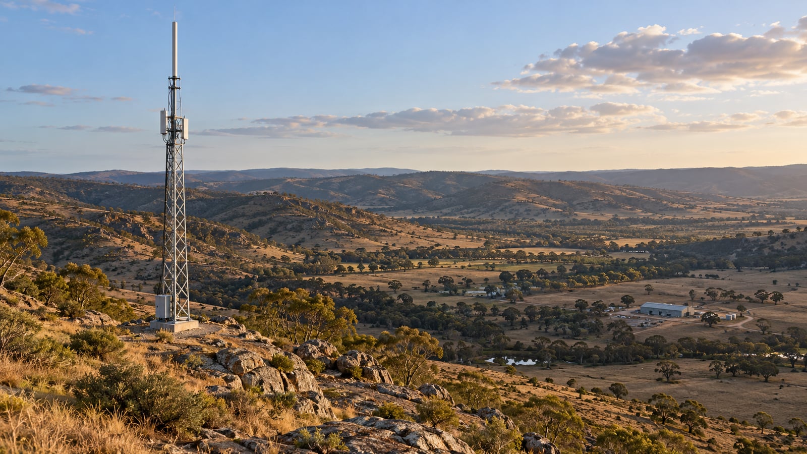
A repeater sits on a hill, its transmitter is running at full power, and the coverage map paints the valley green. The crew gets there and can hear dispatch, but dispatch cannot hear the crew.
That can happen when a prediction uses a vehicle antenna height for handhelds, treats woodland as open ground, or only calculates the stronger direction of the radio link.
A coverage prediction calculates a link budget at many locations. At a weak point, check what caused the loss and whether a different site, height or antenna would improve it before committing to a taller mast or a larger transmitter.
The Short Answer
RF coverage prediction estimates where a radio service will work by combining a propagation model, terrain and clutter data, the antenna system, and a defined receiver requirement. A coverage map is the result of those assumptions at many locations.
Three inputs frequently change its shape:
- Terrain determines which paths are clear, obstructed or beyond the radio horizon.
- Antenna height changes the path over that terrain and the terminal’s position relative to nearby rooftops or tree cover.
- Clutter represents buildings, vegetation and other objects above the ground that affect propagation.
For two-way radio, calculate talk-out and talk-back. The usable service area is where both directions meet the requirement, at the location and time percentages the study actually evaluates.
What an RF Coverage Map Actually Calculates
At one receiver location, the power budget is:
P_rx = P_tx − L_tx + G_tx − L_path + G_rx − L_rx
Power is in dBm, antenna gains are in dBi, and losses are in dB. The transmit and receive losses include the relevant feeder, connector and combining components. The antenna gains must be the gains towards the other terminal, not automatically the largest numbers on the datasheets.
The propagation model supplies the path loss. Check which terrain, clutter and fading effects it already includes before applying separate corrections. Count each loss once.
The planner compares the resulting power with a service threshold. That threshold needs a meaning: a specified voice quality, bit error rate, or other performance target, with the intended receiver and bandwidth. A manufacturer’s sensitivity figure measured under one condition does not automatically define acceptable service in another. Our link budget guide explains the arithmetic in more detail.
Terrain: Why Coverage Does Not Follow a Circle
Two receivers can sit the same distance from a base station and have very different signals. One has a clear path across a valley. The other sits behind the ridge that forms its edge.
Radio energy diffracts into the shadow of an obstruction, so blocked line of sight does not mean zero signal. It does mean additional loss that depends on the path geometry. ITU-R P.526 describes diffraction methods; a complete path calculation must also handle the Earth’s curvature and the propagation conditions assumed for the study.
Start by looking at a terrain profile to a weak point. Identify the obstruction that controls the path before changing the radio equipment. A little more tower height may clear a nearby crest; the same increase may barely change a path blocked by a much higher ridge farther away.
The Terrain Data Viewer can extract those profiles and compare elevation sources. Its clearance view helps inspect the geometry. Frequency-dependent Fresnel clearance and radio loss belong in the Fresnel Zone Calculator, Link Planner or Coverage Predictor.
Bare earth and surface elevation are different inputs
A digital terrain model, or DTM, represents the ground with buildings and vegetation removed. A digital surface model, or DSM, includes the upper surface of those objects as represented by the survey.
Copernicus GLO-30, for example, is a surface model with nominal 30 metre spacing. It is not a bare earth survey. Copernicus explains the distinction here.
That distinction matters when combining data with a model that expects ground elevation and a separate clutter representation. A canopy included in the elevation profile and then added again as a clutter height can describe the same obstruction twice. Check what the propagation method expects and what the elevation source contains.
Antenna Height: Clearance Matters More Than the Mast Number
An antenna height of 30 metres usually means 30 metres above local ground, or AGL. The antenna’s elevation above a common vertical datum also depends on the ground elevation at the site. Mixing those two quantities can move an antenna by hundreds of metres in a calculation.
The height you enter for the receiver is just as important. A handheld at 1.5 metres, a roof-mounted vehicle antenna and a fixed antenna above a shed roof are different coverage cases. If the service is for people on foot, a map calculated for rooftop receivers answers the wrong question.
Raising an antenna changes the line over the terrain. It also changes the elevation angle into the antenna pattern. A higher-gain antenna with a narrower vertical beam needs its actual pattern and mounting tilt checked, especially for users close to a high site.
A 20 metre mast increase does not give every obstacle 20 metres more clearance
Consider a 10 km path at 450 MHz, with both end sites at the same ground elevation. The handheld antenna is 1.5 metres above ground. A narrow ridge halfway along rises 10 metres above the end-site ground level.
At the midpoint, increasing the base antenna from 30 to 50 metres lifts the straight line between the antennas by only 10 metres. The far end has not moved.
Using a fixed effective Earth radius of 4/3 of the physical radius, the midpoint Earth bulge is about 1.47 metres. The first Fresnel zone radius there is:
r₁ = √(λ × d₁ × d₂ / (d₁ + d₂)) ≈ 40.8 m
Here λ is about 0.666 metres and both partial distances are 5,000 metres. A common first clearance check is 60% of that radius, or 24.5 metres.
| Midpoint quantity | 30 m base antenna | 50 m base antenna |
|---|---|---|
| Straight line height above the end-site ground reference | 15.75 m | 25.75 m |
| Ridge height plus effective Earth bulge | 11.47 m | 11.47 m |
| Clearance below the straight line | 4.28 m | 14.28 m |
| 60% first Fresnel zone clearance achieved? | No | No |
The taller mast improves the geometry, but neither case passes that clearance check. Both have geometric line of sight under these assumptions. Seeing over the ridge and clearing enough of the Fresnel zone are different tests.
This is a deliberately simple geometry example, not a complete diffraction prediction. Rounded ridges, other obstructions and a changing atmosphere need the full path model. The radio line of sight guide explains effective Earth radius and the radio horizon.
Clutter: What Happens Around the User
In radio planning, clutter means objects above the terrain, including buildings and vegetation. Its effect depends on the frequency, the surroundings, and where the antennas sit relative to those objects. ITU-R P.2108 provides statistical clutter-loss methods with specific application conditions.
A land-cover map helps identify environments such as tree cover, built-up land, grassland or water. It does not measure the exact height, construction or attenuation of every object in a cell. ESA WorldCover provides global land-cover products for 2020 and 2021 at 10 metre resolution; that is useful context, but it is not a current survey of a growing industrial site.
For a mine or construction project, check the places that may have changed since the source data was acquired: new workshops, stockpiles, cuttings, pit walls and vegetation removal. A detailed-looking raster can still describe an older landscape.
Indoor coverage also depends on building entry loss, the additional loss associated with a terminal inside a building. ITU-R P.2109 models it statistically. This helps with planning across an area, but coverage in a particular basement or behind a particular metal wall needs more site information.
Keep outdoor handheld, indoor handheld and vehicle coverage as explicit requirements. They should not share a legend that quietly changes meaning between them.
Which Propagation Model Should You Use?
Check a model’s frequency, distance and antenna-height limits before using it for the path.
| Method | Useful role in a coverage study | What to check |
|---|---|---|
| Free space path loss | Reference budget for an unobstructed path | It does not describe the losses of a cluttered, obstructed service area. |
| Hata | Empirical land-mobile planning within its published range | Frequency, distance, base and mobile heights, and environment assumptions. |
| NTIA ITM, also called Longley-Rice | Terrain-dependent propagation prediction | Prediction mode, terrain input, variability settings and any separately applied clutter treatment. |
| ITU-R P.1546 | Point-to-area prediction using propagation curves and corrections | Land or sea path, effective antenna height, percentages and the corrections used. |
| ITU-R P.1812 | Path-specific point-to-area prediction using a terrain profile | Terrain and clutter representation, radio-climatic inputs, model edition and percentages. |
NTIA documents ITM for 20 MHz to 20 GHz. The published scopes of P.1546 and P.1812 cover 30 MHz to 4 GHz and 30 MHz to 6 GHz respectively. Those frequency ranges are only part of each method’s applicability.
The noIM₃ Coverage Predictor supports Hata, ITM and ITU-R methods, and records the model used. Keep the model edition and settings with the result. Comparing two maps is much easier when you can establish whether a changed antenna, changed input data or changed propagation method caused the difference.
Worked Example: The Handheld Can Hear but Cannot Answer
Consider a 450 MHz repeater serving a handheld 10 km away. These are illustrative design inputs, not the specifications of a particular radio or measurements from a particular site.
| Input | Base station | Handheld |
|---|---|---|
| Transmitter power | 25 W, rounded to 44 dBm | 5 W, rounded to 37 dBm |
| Antenna gain towards the other end | 8 dBi | −3 dBi |
| Feeder and connector loss | 2 dB | 0 dB |
| Chosen design threshold at the receiver input | −110 dBm | −110 dBm |
The −3 dBi is an assumed effective handheld antenna gain for this exercise. A real study needs an appropriate antenna and body-loss allowance, counted once. The −110 dBm is a chosen design threshold, not a universal DMR, P25 or analogue sensitivity requirement.
The free space reference loss is:
L_FSPL = 32.45 + 20 log₁₀(450) + 20 log₁₀(10) = 105.5 dB
For this arithmetic exercise, suppose an obstructed path has 35 dB of excess terrain loss and 12 dB of additional local clutter loss, giving a total path loss of 152.5 dB. These two losses are stipulated to show the budget, not claimed outputs of a terrain run. With a real propagation model, use its total loss and its documented corrections rather than attaching these numbers to it.
The two budgets are then:
Talk-out: 44 − 2 + 8 − 152.5 − 3 = −105.5 dBm
Talk-back: 37 − 3 − 152.5 + 8 − 2 = −112.5 dBm
| Result | Talk-out: base to handheld | Talk-back: handheld to base |
|---|---|---|
| Received power | −105.5 dBm | −112.5 dBm |
| Margin against the chosen −110 dBm threshold | +4.5 dB | −2.5 dB |
| Meets the threshold? | Yes | No |
Doubling the base transmitter from 25 to 50 watts adds about 3 dB to talk-out. It adds nothing to talk-back. The crew hears a stronger signal and dispatch still cannot hear the crew.
Reducing the path loss by 6 dB, if a revised site or antenna arrangement actually achieves it, improves both budgets by 6 dB. Talk-back would then reach −106.5 dBm, giving 3.5 dB against the chosen threshold. The path model must establish how much improvement a particular site or height change would provide.
Real repeaters normally use different transmit and receive frequencies, and receiver sensitivities, noise and filtering may also differ. Calculate the actual path and equipment in each direction. The shared path loss and threshold here isolate the power imbalance so you can see it plainly.
Map Resolution: More Pixels Do Not Mean More Knowledge
A coverage calculation has several resolutions: the elevation source, land-cover source, path sampling, and spacing between predicted receiver locations. The display adds another layer of interpolation.
Sampling a nominal 30 metre elevation grid every 5 metres does not create a 5 metre survey. It interpolates the existing data. A narrow cutting or a small building may remain unresolved even if the final map looks smooth.
For a polar sweep, spacing also grows with range. Adjacent bearings one degree apart are about 175 metres apart at 10 km, but 524 metres apart at 30 km. Those figures come from distance multiplied by the angle in radians. A finely coloured image between the bearings does not establish what happens in every intervening gully.
Use an overview to compare candidates, then check important routes and weak boundaries at a spacing the input data can support. Record the source and sampling settings with the map.
Reliability: What Does the Coverage Percentage Mean?
Area covered, location reliability and time variability describe different things.
Area coverage is the share of the defined study area that meets the criterion. Location reliability concerns variation between receiver locations within the environment represented by the prediction. Time variability concerns changes over time at a fixed location. The propagation method determines how those statistics are represented and which percentages it supports.
Consequently, a map showing 95% of an area covered does not establish that every radio call succeeds for 95% of the year. Nor does an area statistic establish coverage along the access road, in an emergency assembly area or inside the workshop.
State the service area and the statistical assumptions separately. For an operational network, inspect critical routes and fixed locations as well as the overall percentage. If different models express their variability differently, check those definitions before comparing their legends.
How to Build a Radio Coverage Prediction You Can Check
1. Define the user and the service requirement
Specify the frequency, waveform, bandwidth and performance target. Decide whether the receiver is a vehicle, an outdoor handheld or an indoor handheld, and set its antenna height and losses accordingly. Define the study boundary, critical routes and required locations.
2. Inspect the terrain and data sources
Use the Terrain Data Viewer to inspect profiles towards critical locations. Confirm ground versus surface elevation, source date, resolution and vertical reference. Compare sources where an uncertain ridge or building controls the answer. Recent survey data is particularly valuable where earthworks have changed the site.
3. Enter the complete antenna and radio systems
In the Coverage Predictor, enter each site and service with its actual power, feeder losses, antenna pattern and height. Include the handheld or mobile system and base receiver settings. Use the public tool pages to review the available inputs and outputs before setting up the study.
4. Calculate both directions and inspect the weak points
Review talk-out, talk-back and the worst-of view. At a failure point, inspect the path and loss breakdown. Work out whether the limiting cause is terrain, terminal clutter, an antenna pattern, receiver performance or interference. Increasing power is only useful when it improves the limiting budget.
5. Compare one design change at a time
Keep the model, study boundary and service criterion consistent while comparing tower heights, site positions or antennas. A difference map helps show where a change buys useful coverage and where it does little. A new site that fills a critical shadow may be more valuable than a larger overall coverage area elsewhere.
6. Validate with measurements and retain the assumptions
Import suitable drive-test measurements and check the residuals, not just how closely the colours appear to match. Compare like with like: frequency, receiver quantity, antenna, height and measurement setup. Use separate measurements to assess a calibrated model where possible; testing only the points used to fit it gives an optimistic view of its predictive accuracy.
Export the report and GIS layers with the radio configuration, model editions, data sources, grid spacing, thresholds and reliability settings. A colleague should be able to tell what the map means without reconstructing the project from memory.
How Accurate Is RF Coverage Prediction?
There is no single accuracy figure that applies to every coverage map. Error depends on the propagation method, terrain and clutter inputs, the radio configuration and how well those represent the actual site.
A useful validation reports bias and scatter. Mean error shows whether predictions are systematically high or low. Root mean square error, or RMSE, captures the size of the residuals and is sensitive to large misses. An overall average can hide poor results in one environment, so also inspect residuals by land cover, route and signal level.
The Coverage Predictor can import drive-test data and report validation statistics. Calibration can correct a systematic offset; it cannot restore a missing ridge, turn old land cover into a current site survey or establish coverage inside a building that was never measured.
Frequently Asked Questions
What is RF coverage prediction?
RF coverage prediction estimates received signal or service performance across an area using a propagation model, terrain and clutter data, and the radio and antenna systems. Its result depends on the receiver requirement and the statistical conditions stated with the map.
How does terrain affect radio coverage?
Terrain changes path clearance, diffraction and the radio horizon. A receiver behind a ridge can have much greater path loss than another receiver at the same distance on a clear path. Inspecting a profile helps identify which obstruction controls the result.
Does increasing antenna height always improve coverage?
It often improves clearance, but the benefit depends on where the obstruction sits and how the antenna pattern illuminates the service area. A height change at one end gives progressively less additional straight-line clearance towards the unchanged end of the path. Recalculate the actual geometry.
What is clutter in RF planning?
Clutter means objects above the terrain, including vegetation and buildings. Land-cover classes help represent the environment statistically. They are not exact measurements of individual building materials, tree heights or local obstructions.
Why can I hear the repeater when it cannot hear me?
The base station may transmit substantially more power than a handheld. Different receiver sensitivities, antenna losses, interference and noise also affect the two directions. Check talk-back separately; increasing the base transmitter power only improves talk-out.
Is a line of sight map the same as a radio coverage map?
No. A line of sight map describes visibility under its geometry assumptions. A radio coverage map also needs frequency-dependent propagation loss, antenna patterns, equipment losses and a receiver criterion. Some obstructed paths still work through diffraction, while some visible paths fail the service requirement.
Does a smaller prediction grid make the map more accurate?
A smaller grid resolves changes between calculation points more closely, but cannot improve the native resolution or age of the input data. It can help reveal a weak boundary while leaving the underlying terrain or clutter uncertainty unchanged.
Try the Numbers
Start with the Terrain Data Viewer to understand the ground and the source data. Use the Coverage Predictor to compare sites and antenna systems, inspect both directions and validate against measurements. The Link Budget Calculator and Fresnel Zone Calculator let you check the individual budgets and clearance calculations along the way.
For the foundations behind the map, see free space path loss, antenna gain and radiation patterns, and the noise floor and receiver sensitivity.
Notes on Sources
The 450 MHz budgets, mast-height comparison and bearing-spacing figures are our own arithmetic using the assumptions stated in each example. The 35 dB terrain and 12 dB clutter losses are illustrative inputs, not measurements or claimed outputs of a noIM₃ coverage study. No measured accuracy or achieved coverage percentage is claimed for an actual site.
- ITU-R P.526, Propagation by diffraction, for diffraction methods and Fresnel-zone geometry. The 60% clearance check is a planning rule used here to illustrate the difference between visibility and clearance, not a service guarantee.
- NTIA, Irregular Terrain Model (ITM), Longley-Rice, for the model’s scope and its treatment of terrain and variability.
- ITU-R P.1546 and ITU-R P.1812, for point-to-area prediction methods and their published scopes. Use the edition recorded with the software result when reproducing a study.
- ITU-R P.2108, Prediction of clutter loss, and ITU-R P.2109, Prediction of building entry loss, for the distinction between terminal clutter and indoor loss.
- Copernicus Data Space, Copernicus DEM, for the surface-model definition and GLO-30 spacing; ESA WorldCover, for the land-cover product dates and resolution.