Antenna Utilities

Parabolic Antenna Calculator

Dish antenna gain, beamwidth, and aperture analysis for satellite, microwave, and radio astronomy systems. From reflector diameter, frequency, and efficiency to gain in dBi, half power beamwidth, effective aperture, and far field distance.

Overview

Parabolic dish antennas dominate every link where high gain in a small angular footprint matters. Satellite ground stations, microwave backhaul, point to point millimetre wave, radar, radio astronomy, deep space communications. The physics is the same in every case. A reflector of diameter D collects energy across its physical aperture and focuses it into a narrow beam. Realised gain follows G equals eta times pi D divided by lambda all squared, where lambda is the wavelength and eta is the antenna efficiency. The half power beamwidth follows roughly 70 lambda over D in degrees. From those two relationships every other parameter that engineers actually use (effective aperture, far field distance, pointing tolerance) falls out.

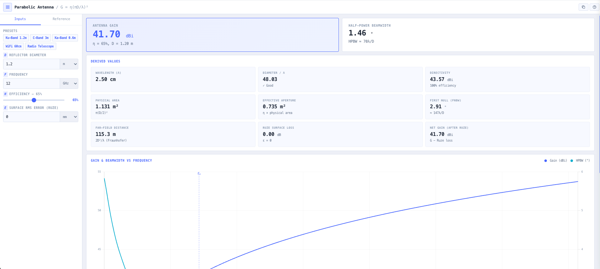
The noIM₃ Parabolic Antenna Calculator computes every one of those parameters from the inputs that engineers actually have on hand. Reflector diameter in metres. Operating frequency in GHz. Antenna efficiency as a percentage with guidance for the common feed configurations (prime focus, offset, Cassegrain). The output is realised gain in dBi alongside theoretical directivity in dBi (so you can see how much performance the feed system is costing you), half power and first null beamwidths in degrees, effective aperture and physical area, far field (Fraunhofer) distance in metres, and the diameter to wavelength ratio that determines whether the reflector is electrically large enough to deliver the gain you want.

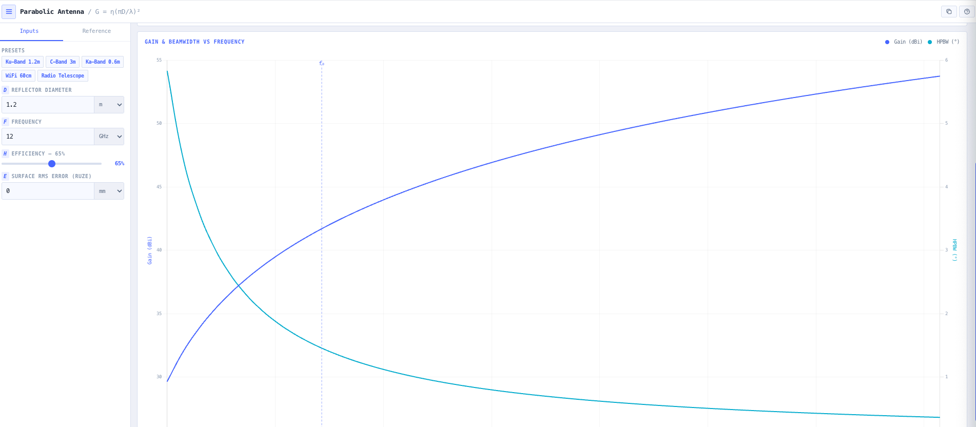
A gain versus frequency sweep visualisation shows how performance scales across bands, which is the right way to evaluate a dish upgrade from C band to Ku band, or to validate that a microwave backhaul antenna keeps its gain across the operator licensed channel range. Built in presets for a Ku band 1.2 m dish, a C band 3 m dish, a Ka band 0.6 m dish, a 60 cm WiFi grid antenna, and a 25 m radio telescope accelerate common workflows. Browser only computation means design data never leaves the machine, which matters for defence, intelligence, and commercially confidential satellite work.

Capabilities

Gain and directivity calculation

Realised gain in dBi from reflector diameter, wavelength, and efficiency using G equals eta times pi D over lambda squared. Theoretical directivity in dBi shown alongside so the cost of feed inefficiency is explicit. Diameter to wavelength ratio surfaced to indicate whether the reflector is electrically large enough at the operating frequency.

Half power and first null beamwidth

Computes half power beamwidth (HPBW) and first null beamwidth from the standard parabolic relationships. HPBW is essential for satellite alignment tolerance, link pointing sensitivity, interference coordination, and pencil beam radar applications. First null beamwidth supports adjacent satellite interference analysis on geostationary arcs.

Effective aperture and physical geometry

Effective aperture in square metres alongside physical reflector area, wavelength, and diameter to wavelength ratio. Useful for system level modelling, link budget calculations that take antenna gain from physical geometry rather than vendor datasheet, and visualising the electrical to physical scaling as frequency changes.

Adjustable efficiency for common feeds

Antenna efficiency (eta) is configurable with guidance for prime focus (typically 50 to 60 per cent), offset feed (typically 65 to 75 per cent), and Cassegrain (typically 60 to 70 per cent) configurations. Allows realistic performance modelling that accounts for spillover, aperture blockage, illumination taper, and feed loss.

Far field (Fraunhofer) distance

Computes the far field boundary at 2 D squared over lambda, which sets the minimum range at which the radiation pattern is fully formed. Critical for antenna range measurements, near field exclusion zone calculations, and confirming that the link distance places the receive antenna in valid far field for the operating frequency.

Ruze surface error loss

Optionally enter a surface RMS error to apply the Ruze equation, delta G equals exp of minus 4 pi epsilon over lambda all squared. The calculator reports the surface error loss in dB and the net gain after that loss. Surface tolerance scales with frequency, so this is the constraint that sets the usable upper band of a given reflector.

Frequency sweep visualisation

Gain and HPBW versus frequency shown as a sweep across the operating band so multi band design decisions can be evaluated visually rather than through repeated point calculations. Useful for validating that an antenna keeps its gain across the operator licensed channel range, and for evaluating dish upgrades from one band to another.

Band presets

Quick select presets for a Ku band 1.2 m dish at 12 GHz, a C band 3 m dish at 4 GHz, a Ka band 0.6 m dish at 20 GHz, a 60 cm WiFi grid antenna at 5.8 GHz, and a 25 m radio telescope at 1.4 GHz accelerate common workflows. Manual entry remains available for unusual frequencies, deep space and millimetre wave applications, or sub GHz reflector work.

Browser only computation

Runs entirely in your browser. No reflector geometry, frequency, or design data is submitted to a server. Useful for defence, intelligence, and commercially confidential satellite ground segment work, or any environment where information security policy prohibits sending engineering data to third party services.

Standards & methodology

  • IEEE 145. Standard definitions of terms for antennas
  • ITU R BO.1213. Reference radiation patterns for satellite earth station antennas
  • ITU R S.580. Radiation diagrams for use as design objectives for antennas of earth stations
  • ETSI EN 302 217. Fixed radio systems antenna characteristics for fixed point to point links
  • ACMA radiocommunications licence conditions referencing antenna performance and beamwidth

When to use this tool

  • Designing satellite ground station antennas across C, X, Ku, and Ka bands
  • Microwave backhaul link planning and antenna selection
  • Evaluating dish upgrades from one band to a higher frequency band
  • Assessing beamwidth for adjacent satellite interference coordination on the geostationary arc
  • Validating manufacturer datasheet gain against the physics from diameter and frequency
  • Calculating far field distance for antenna range measurements and pattern testing
  • Quantifying the Ruze surface error loss when assessing a dish for a higher frequency band
  • Radio astronomy and deep space communications reflector analysis
  • Producing antenna performance evidence for ACMA microwave licence applications
  • Comparing prime focus, offset, and Cassegrain feed configurations for the same reflector
  • Sizing dish diameter to meet a required gain target at a given frequency
  • Teaching parabolic antenna fundamentals and the diameter to wavelength relationship
  • Sanity checking vendor proposed antenna performance against independent calculation

Is this the right tool for you?

Reach for the Parabolic Antenna Calculator in any of the following situations.

  • You are sizing a satellite ground station antenna for a C, X, Ku, or Ka band uplink or downlink and need realised gain in dBi from physical geometry rather than relying on a vendor datasheet.
  • You are planning a microwave backhaul link and need to confirm the proposed dish diameter delivers the gain required by the link budget at the operating frequency.
  • You are evaluating whether an existing dish can be reused at a higher frequency band (for example C to Ku, or Ku to Ka) and need to see how gain and beamwidth scale across the new band.
  • You are coordinating against adjacent satellite interference on the geostationary arc and need accurate first null beamwidth to validate angular separation against the operator standard.
  • You are validating manufacturer datasheet gain claims against the physics from diameter, frequency, and feed efficiency before accepting a procurement.
  • You need the far field (Fraunhofer) distance to plan an antenna range measurement campaign, set up a near field exclusion zone, or confirm a link is operating in valid far field at the receive end.
  • You are working on radio astronomy or deep space communications reflector analysis and need precision gain, beamwidth, and effective aperture across very large diameter to wavelength ratios.
  • You are producing antenna performance evidence for an ACMA microwave licence application and need defensible engineering output showing gain and beamwidth at the licensed frequency.
  • You are comparing prime focus, offset, and Cassegrain feed options for the same reflector and want to see how realistic efficiency assumptions change the realised gain.
  • You are sizing a dish to meet a target gain at a known frequency and want a fast solver rather than iterating through manufacturer catalogues.
  • You are pointing a satellite dish in the field and want to know the half power beamwidth so you understand the alignment tolerance the link can survive.
  • You are training new RF engineers in parabolic antenna fundamentals and want a teaching tool that shows the diameter to wavelength relationship driving gain and beamwidth.
  • You are evaluating millimetre wave point to point antennas where small diameter to wavelength ratios fall apart and need to confirm the reflector is electrically large enough.
  • You are a consulting engineer producing antenna analysis for a customer report and need engineering grade outputs rather than vendor brochure summaries.
  • You are operating under a security regime that prohibits sending design data to third party services and need a calculator that runs entirely in your browser.

Frequently asked questions

What formula does the calculator use?

Realised gain follows G equals eta times pi D divided by lambda all squared, where D is the reflector diameter, lambda is the wavelength, and eta is the antenna efficiency. Theoretical directivity is the same expression with eta set to one. Half power beamwidth follows the standard relationship of approximately 70 lambda over D in degrees. Far field distance follows 2 D squared over lambda. All formulas are aligned with IEEE 145 standard definitions and the satellite earth station references in ITU R BO.1213 and S.580.

What antenna efficiency should I use?

Efficiency depends on the feed configuration. Prime focus dishes typically run 50 to 60 per cent. Offset feed dishes typically run 65 to 75 per cent. Cassegrain dishes typically run 60 to 70 per cent. High performance precision antennas can exceed these ranges, while imperfect surface tolerance, feed misalignment, or aperture blockage can drag efficiency down. The calculator accepts efficiency as a percentage so you can model the configuration you actually have, and a separate surface RMS error input applies the Ruze surface loss on top.

What is HPBW and why does it matter?

Half power beamwidth (HPBW) is the angular width across which the antenna gain drops by 3 dB from the boresight peak. It defines the alignment tolerance your link can survive, the angular separation needed for adjacent satellite interference coordination, and the pointing sensitivity required for satellite tracking systems. A 1.2 metre Ku band dish has roughly 1 degree HPBW. A 2.4 metre Ka band dish has roughly 0.25 degrees. Tighter beamwidth means better gain but tighter pointing requirements.

Why does the diameter to wavelength ratio matter?

Parabolic antenna theory assumes the reflector is electrically large, meaning D divided by lambda is large. As D over lambda approaches small values (typically below 10 to 15), the gain formula starts to over predict because edge diffraction and aperture phase errors become significant. The calculator surfaces D over lambda directly so you can confirm the reflector is electrically large enough at the operating frequency before relying on the predicted gain.

What is the Fraunhofer distance and when do I need it?

The Fraunhofer (far field) distance is 2 D squared divided by lambda. It is the minimum range at which the radiation pattern is fully formed and the gain formula is valid. Closer than this, you are in the near field, where the field structure is more complex and the simple gain formula does not apply. Critical for antenna range measurements, near field exclusion zone calculations for human exposure, and confirming that a link distance places the receive antenna in valid far field.

What is Ruze surface error loss?

A real reflector deviates from a perfect paraboloid. The Ruze equation gives the resulting gain loss as delta G equals exp of minus 4 pi epsilon over lambda all squared, where epsilon is the surface RMS error. Because the error is measured against the wavelength, the loss climbs steeply with frequency, which is why a dish that performs well at C band may be unusable at Ka band. Enter a surface RMS error and the calculator reports the loss in dB and the net gain after it. A common design target is to keep epsilon below lambda divided by 20.

How do I evaluate a dish for use at a higher frequency band?

Use the frequency sweep visualisation. The same physical reflector at a higher frequency has a smaller wavelength, so the diameter to wavelength ratio increases, gain increases (approximately as frequency squared), and HPBW shrinks (approximately as 1 over frequency). Surface tolerance also becomes more critical at higher frequencies, and feed efficiency typically drops, both of which work against the gain increase. The calculator shows the predicted gain and beamwidth across the new band so the trade off is visible.

Does any data leave my browser?

No. The calculator runs entirely in your browser. No reflector geometry, frequency, or design data is submitted to a server. Useful for defence, intelligence, and commercially confidential satellite ground segment work, or environments where information security policy prohibits sending engineering data to third party services.

Does it cover offset and Cassegrain feeds?

Yes. Efficiency input accepts the realistic value for offset and Cassegrain configurations, and the calculator returns realised gain accordingly. The underlying gain physics is the same across feed types because the aperture is the same. The differences show up in efficiency (Cassegrain and offset typically beat prime focus by a few per cent) and in the radiation pattern detail, which is beyond the scope of the gain and beamwidth calculation but supported by the noIM₃ Antenna Builder for full pattern modelling.