Terrain aware land mobile radio coverage prediction on a polar grid, with Hata, the NTIA reference ITM, ITU-R P.1546 and P.1812, P.526 diffraction, P.2108 clutter and P.2109 building entry loss, calibrated against your own drive test data.
Included in the 14-day Pro trial on every new account. No credit card.
Coverage Predictor
6 inputs→8 outputs
Walkthrough
See it working
Coverage Predictor1 / 9
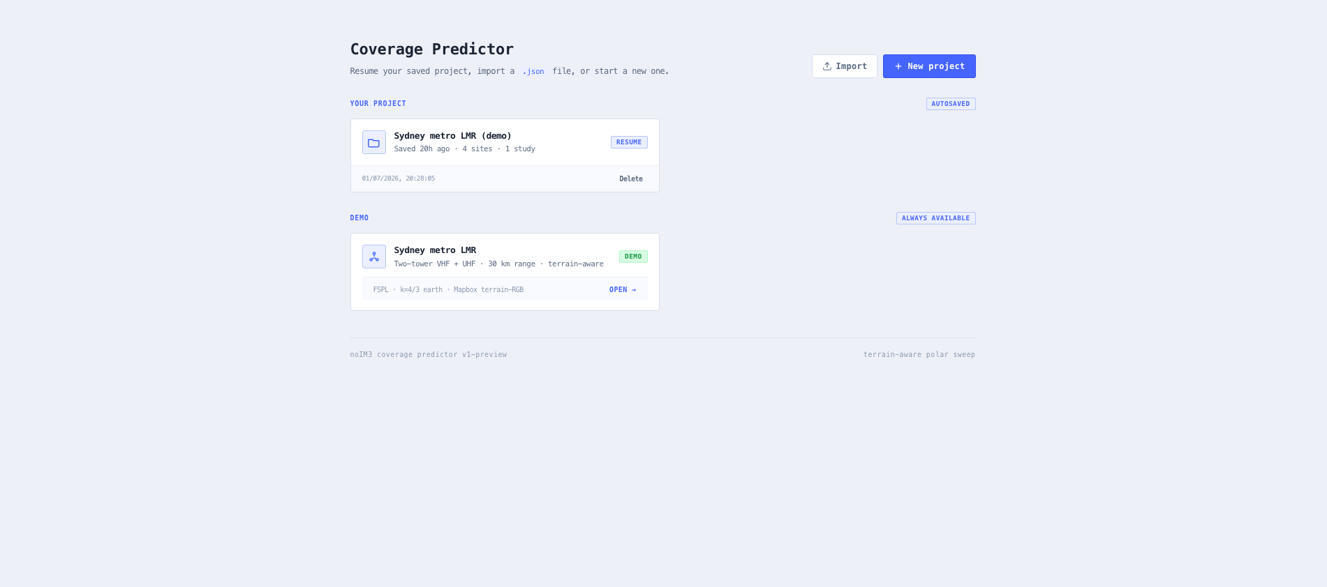
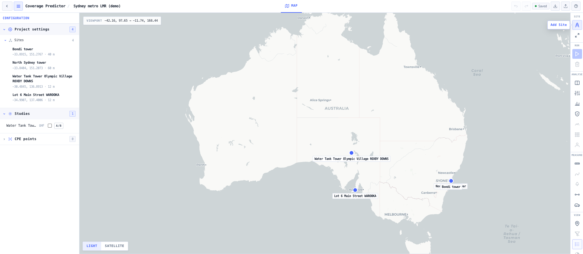
Project tree on the left, map in the centre, grouped tool rail on the right, geometry status bar along the bottom.
Overview
What the Coverage Predictor does
Coverage prediction is easy to do badly. Pick a model, feed it a distance, and you get a number that looks like an answer. The number is worth something only if you can say which model produced it, whether the inputs were inside the range that model was fitted over, how much of the result is terrain and how much is a fade margin, and how far the prediction sat from reality the last time anyone drove the area with a receiver. This tool is built so every one of those questions has an answer attached to the cell you are looking at.
Read the full overview
Prediction runs as a polar sweep centred on the tower. For each bearing and ring the engine samples a terrain profile from the global DEM, applies earth curvature at a standard atmosphere effective earth radius, and resolves the chord against a propagation model chosen for that chord rather than for the whole study. Hata Okumura and COST 231 are used inside their published validity envelope. Outside it the engine falls back to the NTIA reference Irregular Terrain Model, which is valid from 20 MHz to 20 GHz and is the model behind regulatory coverage submissions in many jurisdictions. ITU-R P.1546 and P.1812 are available on the same footing. Whichever is used is recorded, per cell and in the run manifest, and can be forced for a sensitivity study.
What sits on top of the base model matters as much as the base model. Knife edge diffraction is layered onto bearings where the line of sight is blocked, so those cells carry a realistic fade margin instead of a null. Clutter height gain corrects for a terminal below rooftop or canopy top. Building entry loss converts an outdoor field strength into an indoor prediction for the handheld that is actually inside the building. And because no propagation model removes the residual against reality, drive test data is ingested as a measured residual and propagated through the per cell uncertainty, so the confidence figure on screen reflects your own measurements rather than a textbook sigma.
Capabilities 10
Polar sweep over terrain accurate path profiles
Coverage is predicted on a polar grid centred on the tower. Every bearing and ring cell samples its own terrain profile from the Mapbox global Terrain RGB DEM at a configurable density, applies earth curvature at a standard atmosphere effective earth radius following ITU-R P.530, and resolves the chord independently. Rasterisation runs off the main thread so the map stays responsive while a study lands.
Automatic propagation model selection, recorded not hidden
Hata Okumura and COST 231 are used when the chord sits inside their published validity: 150 to 2000 MHz, base height 30 to 200 m, mobile height 1 to 10 m, range to 20 km. Outside that the engine falls back to the NTIA reference Irregular Terrain Model, valid from 20 MHz to 20 GHz. ITU-R P.1546 and P.1812 are available on the same terms. The decision is recorded in the run manifest and preserved on each cell, and either model can be forced for a sensitivity study.
Diffraction, clutter, vegetation and building entry as explicit layers
ITU-R P.526 single knife edge diffraction with a mid path bulge approximation is applied to blocked bearings so they receive realistic fade margins rather than nulls. P.2108 clutter height gain corrects for terminals below rooftop or canopy top, keyed on ESA WorldCover land cover sampled per profile point. P.833 adds depth aware woodland loss over forest cells, bounded so it never double counts the representative clutter. P.2109 building entry loss converts outdoor field strength to an indoor prediction for traditional or thermally efficient construction at a percentile you set. Each contribution stays separately visible in the cell loss stack.
Measured antenna library with pattern preview
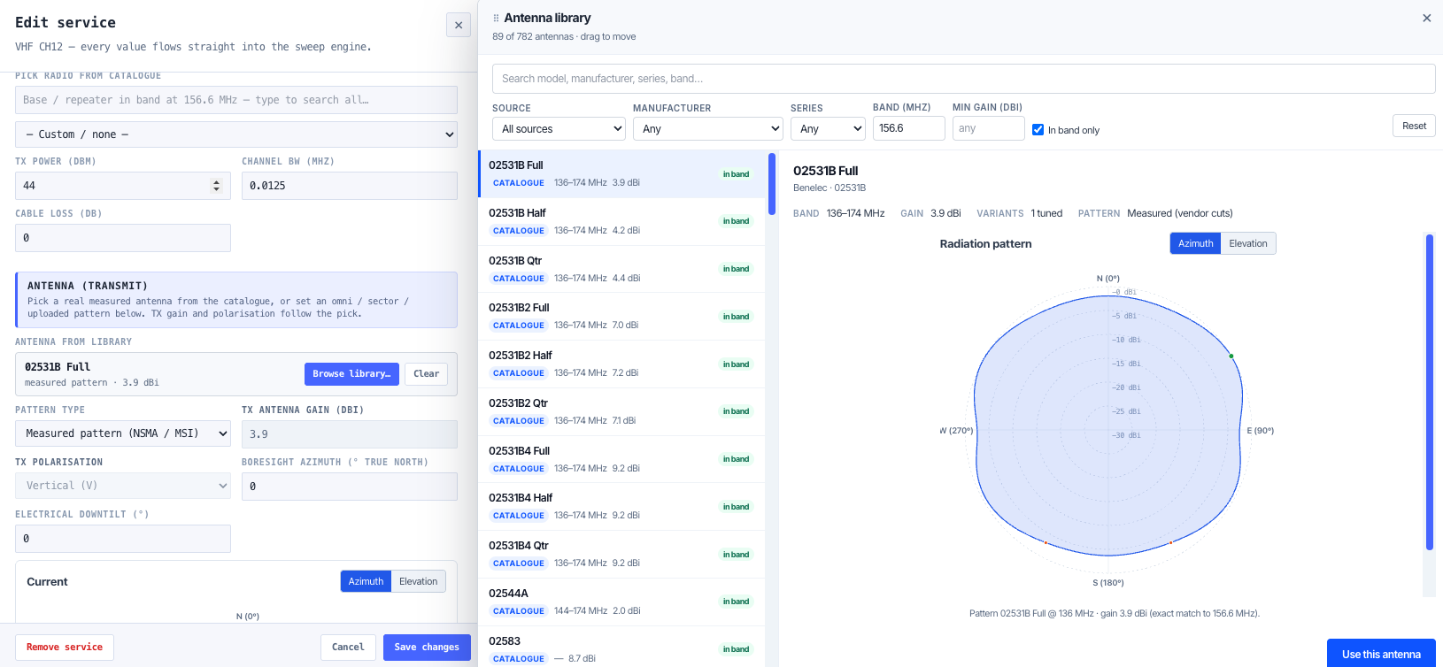
Set a service antenna from a filterable library of real measured antennas rather than a generic omni or sector. Filter the whole catalogue by search text, source, manufacturer, series, band and minimum gain, with in band antennas floated to the top for the service frequency, preview the azimuth and elevation radiation pattern before you commit, and apply the vendor gain, polarisation and measured pattern in one click so the directional sweep uses the real pattern.
One study, many views
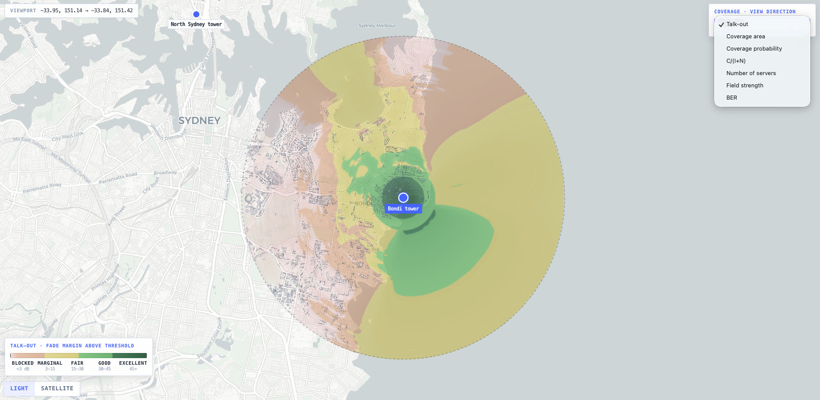
A single sweep re renders into talk out, talk back and worst of, which is the two way usable coverage an integrator actually signs off. Coverage area is a binary mask, coverage probability shows per cell confidence against the combined uncertainty, C over I plus N exposes multi site interference, number of servers highlights hand off zones, field strength in dBuV per metre supports contour filings, and BER covers TETRA, P25, DMR, NXDN and analogue FM. Multi site simulcast networks add simulcast receive and delay spread. Switching views does not re run the engine.
Drive test calibration folded into the uncertainty
Measured field readings import from generic CSV or NMEA, with auto detection of TEMS Investigation, Nemo Outdoor and JV Mobile exports. The engine computes the residual against the prediction and applies either a constant offset or a per-environment bias and sigma bucketed by land cover, with a hold-out accuracy check so the fit is not flattering itself, and propagates the residual sigma through the per cell uncertainty quadrature so the reported combined sigma reflects measured residual. A validation pack reports mean error, RMSE, sigma, correlation, the measured-versus-predicted regression and percent within 6, 10 and 15 dB, overall and per clutter class, and exports a reproducible CSV. The calibration state travels in the run manifest.
Two reliability percentiles that are not the same thing
Location reliability drives the lognormal slow fading margin and models the spatial distribution of users within a cell. Time reliability is orthogonal and covers the fraction of time a link clears its threshold at a fixed point. On the empirical base models the time variability sigma is an internal engineering estimate rather than an ITU validated figure, and it is disclosed as such in the run manifest rather than presented as a published number. The ITM and P.1812 paths use their own published time variability.
Per cell provenance
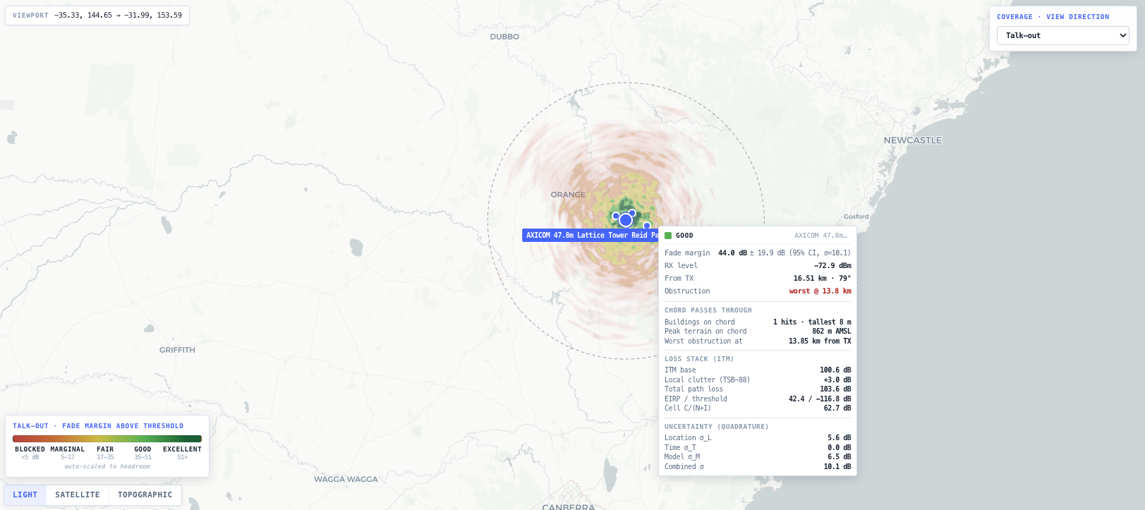
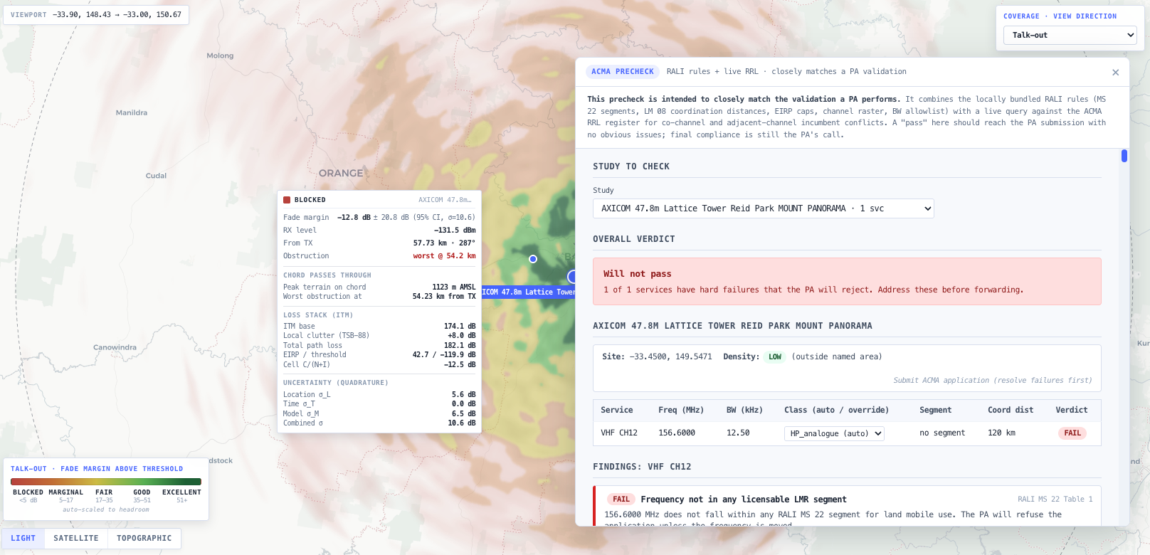
Hover any cell for its received level, fade margin, tier, distance and bearing, the full loss stack from base model through diffraction, clutter, building entry and body loss, and the combined sigma from the uncertainty quadrature. This is what makes a prediction arguable rather than a colour on a map, and it is what survives into every export.
Comparison, optimisation, frequency planning and ACMA precheck
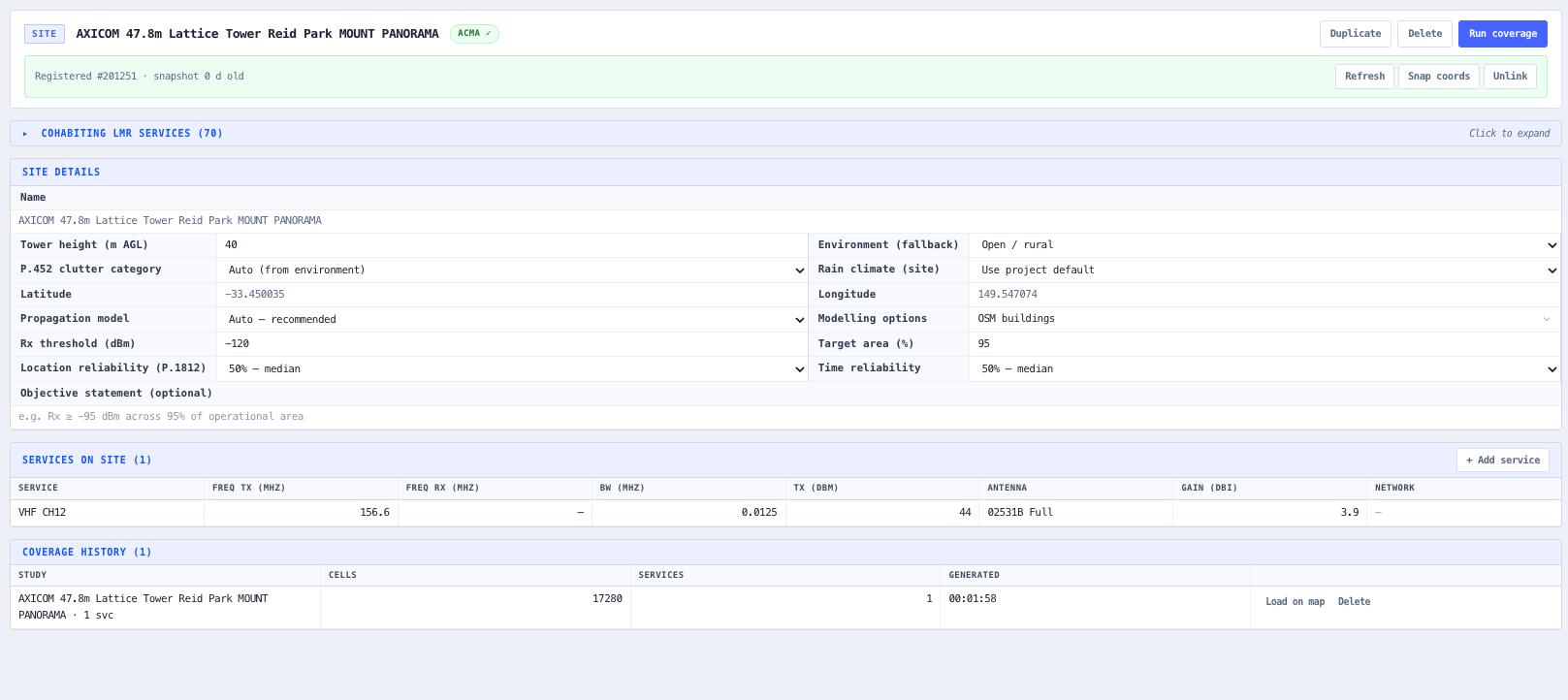
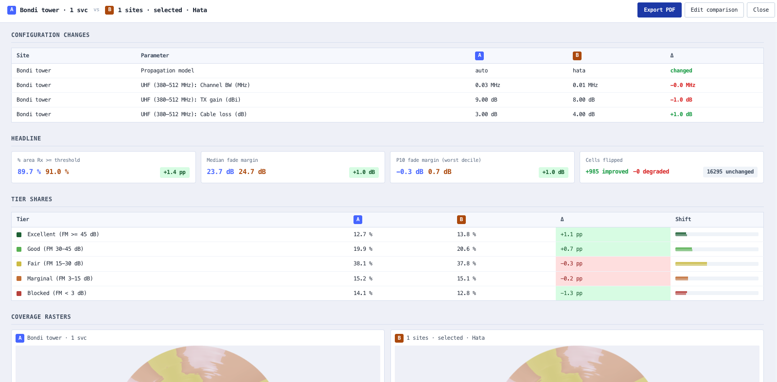
The comparison workspace diffs two studies with a coverage delta raster and area statistics for alternate site, height or service mix work. The optimiser sweeps candidate tower heights, tilts and azimuths and ranks them against a coverage objective. The frequency plan workspace builds a network wide channel matrix and flags reuse conflicts by carrier to interference severity. The regulatory workspace runs an ACMA precheck against the bundled RALI rules and the live RRL.
Models cross checked against independent implementations
The propagation models are validated against executable reference code rather than hand transcribed tables: eeveetza Py1546, Py1812 and Py452 from the ITU-R SG3 rapporteur, itmlogic for Longley-Rice, and ITU-Rpy for rain, with reference outputs committed as fixtures the test suite checks against. The composition from terrain sample through model selection, diffraction, clutter and tiering is proven end to end by test.
Inputs and outputs
What goes in, what comes out
Inputs 6
Site position and tower height above ground level, with ground elevation sampled from the terrain DEM
Land mobile service presets for VHF Lo, VHF Hi, UHF, 700, 800 and 900 MHz, each carrying TX power, antenna gain, feeder loss, RX noise figure, RX height and body or mismatch loss
Antenna as omni, sector, an imported NSMA, MSI or Cambium radiation pattern, or a measured antenna picked from the filterable catalogue library
Sweep geometry: range to 50 km, ring count, bearing count, chord sampling precision and compute mode
Hata environment class, location reliability percentile, time reliability percentile, rain climate and time percentage
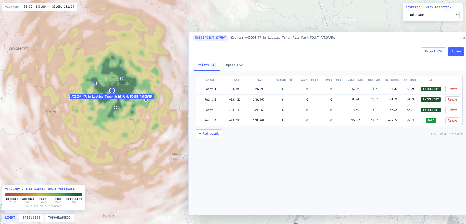
Optional drive test measurements from CSV or NMEA, and CPE or IoT receiver points for a multipoint study
Outputs 8
Tiered coverage heat map, graded Excellent, Good, Fair, Marginal or Blocked against the receiver threshold
Per cell received level, fade margin, loss stack, propagation model used and combined sigma
Talk out, talk back, worst of, coverage area, coverage probability, C over I plus N, number of servers, field strength and BER views
Simulcast receive level and delay spread on multi site simulcast networks
Per point link budgets for fixed CPE or IoT receivers from the multipoint study
Coverage delta rasters and area covered statistics between two scenarios
A validation pack of measured-versus-predicted accuracy metrics, overall and per clutter class, exported as CSV
High resolution coverage KMZ for Google Earth with a legend, georeferenced GeoTIFF raster and GeoJSON vector for GIS, plain KML, CSV, a project round trip to JSON, and a machine readable run manifest; sites also bulk import from CSV or GeoJSON
Standards & methodology
ITU-R P.1546 and ITU-R P.1812 point to area propagation, cross checked against the SG3 rapporteur reference code
NTIA reference Irregular Terrain Model, 20 MHz to 20 GHz, cross checked against itmlogic
Hata Okumura and COST 231 within their published validity envelope
ITU-R P.526 knife edge diffraction with mid path bulge approximation
ITU-R P.2108 clutter height gain and ITU-R P.2109 building entry loss
ITU-R P.833 woodland loss and TIA TSB-88-B Table 19 clutter, keyed on ESA WorldCover land cover
ITU-R P.452 interference and ITU-R P.372 man made noise
ITU-R P.530 and P.838 rain attenuation, with the effective earth radius convention of P.530
ACMA RALI rules and the live Register of Radiocommunications Licences for the coordination precheck
Use cases
When to use this tool
01Designing greenfield land mobile coverage for public safety, utility, mining, defence or transport networks
02Validating an existing repeater or simulcast site against current terrain, clutter and reliability targets
03Comparing candidate tower positions side by side against a target coverage objective
04Calibrating a prediction against drive test data so the confidence figure reflects measured residual
05Predicting indoor handheld coverage with building entry loss rather than assuming an outdoor result holds inside
06Solving per point link budgets for fixed CPE or IoT receivers across a service area
07Building a network wide frequency plan and resolving co-channel reuse before a licence application
08Deciding between more transmit power, a taller antenna, or another site to close a coverage hole
09Running an ACMA coordination precheck against incumbent licences before preparing a submission
10Producing coverage overlays for tender submissions, customer engineering packs and field crews, as Google Earth KMZ or GIS GeoTIFF and GeoJSON
Whichever one is defensible for that chord. Hata Okumura and COST 231 are used inside their published validity envelope of 150 to 2000 MHz, base height 30 to 200 m, mobile height 1 to 10 m and range to 20 km. Outside that envelope the engine falls back to the NTIA reference Irregular Terrain Model, valid from 20 MHz to 20 GHz. ITU-R P.1546 and P.1812 are available on the same footing. The choice is recorded per cell and in the run manifest, and you can force a model for a sensitivity study.
How accurate is the prediction?
The models themselves are cross checked against independent executable reference implementations, and the composition through terrain, diffraction, clutter and tiering is proven by test, so the number on screen matches the loss stack behind it. What no propagation tool can remove is the residual against reality at your particular site. That is why drive test ingestion exists: the measured residual sigma is propagated through the per cell uncertainty, so a calibrated study reports confidence based on your own measurements rather than a textbook figure.
What is the difference between location reliability and time reliability?
Location reliability covers the spatial spread of users within a cell and drives the lognormal slow fading margin added on top of the median prediction. Time reliability covers the fraction of time a link clears its threshold at one fixed point, under tropospheric and multipath variability. They are independent and both are configurable. On the empirical base models the time variability sigma is an internal engineering estimate rather than an ITU validated figure, and the run manifest says so rather than dressing it up.
Can it predict indoor coverage?
Yes, through ITU-R P.2109 building entry loss, which converts the outdoor field strength into an indoor prediction for traditional or thermally efficient construction at a percentile you choose. It is a statistical building entry model rather than a per building one, so it answers whether handhelds inside typical construction in an area will work, not what happens in one specific basement.
What does talk back mean, and why does worst of matter?
Talk out is the downlink from the tower to the mobile. Talk back is the uplink, which is usually the weaker direction because a handheld transmits at a fraction of a base station power. Worst of is the intersection, and it is the honest answer to whether a user has two way communications at that point. Predicting only talk out overstates a network, which is why the tool renders all three from one sweep.
Does it produce a PDF engineering report?
Not yet. Today the tool exports a high resolution coverage KMZ for Google Earth (heatmap overlay plus legend), a georeferenced GeoTIFF raster and a GeoJSON vector layer for GIS, plain KML, CSV, a full project round trip to JSON, and a machine readable run manifest that records model selection, terrain sampling, calibration state and percentile choices. A long form PDF engineering report is in development.
What happens when several services are layered on one tower?
The per service rasters merge by picking the strongest available service in each bearing and ring cell, which reflects what a mobile would actually achieve there rather than averaging across bands that propagate very differently. The merge decision is preserved on the cell, so the contribution breakdown still identifies which service drove the prediction.