RF Utilities

Minimum Detectable Signal Calculator

Receiver sensitivity and minimum detectable signal for RF systems integration. Compute the MDS from bandwidth, noise figure, and required SNR, audit a datasheet sensitivity, add spread-spectrum processing gain, and turn the threshold into detection margin and range.

Free forever on a Standard account. No credit card.

Overview

The minimum detectable signal is the single most important number about a receiver: the weakest signal at its input that still produces a usable output. It is the receiver noise floor plus the signal to noise ratio the demodulator needs, and the noise floor is the thermal noise in the channel raised by the receiver noise figure. Written out, MDS equals −174 dBm/Hz plus 10·log₁₀ of the bandwidth plus the noise figure plus the required SNR. Every term matters, and the mistakes come from dropping one of them or mixing up the bandwidth.

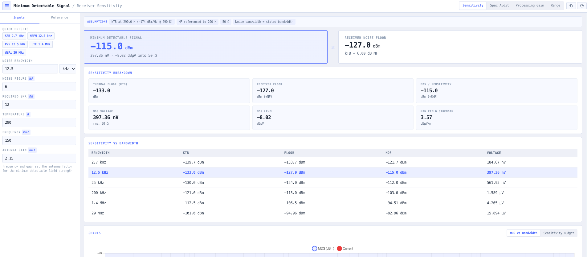
The noIM₃ Minimum Detectable Signal Calculator is the sensitivity utility for that work, written for a systems integrator rather than a circuit designer. The noise figure and required SNR are inputs taken from datasheets and modulation tables, not synthesised, and the output is framed as the numbers that appear in the field. The Sensitivity mode reports the MDS as a power in dBm, as an rms voltage and a dBµV level across 50 Ω that can be dialled straight into a signal generator, and as a minimum detectable field strength in dBµV/m through the antenna factor, so the same threshold reads against a bench source, a spectrum analyser marker, or a field strength limit.

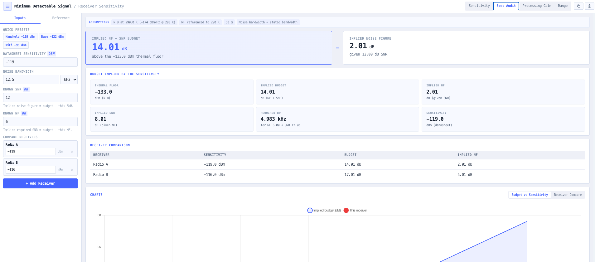
Beyond the forward calculation the tool does the three jobs that surround it. Spec Audit reverse-solves a datasheet sensitivity into the noise figure and SNR budget it implies, flags a figure that is physically impossible for its bandwidth, and compares receivers on a like for like basis. Processing Gain covers spread spectrum, where a direct sequence, GPS, or LoRa waveform is recovered below the thermal noise floor by the processing gain Gp = 10·log₁₀(BW ÷ R). Range turns the threshold into an operational answer: the received signal against the MDS gives a detection margin, and the maximum free space range is solved from the path loss the link can tolerate.

Capabilities

MDS from bandwidth, noise figure, and required SNR

Compute the minimum detectable signal as MDS = −174 dBm/Hz + 10·log₁₀(B) + NF + SNR, with the thermal floor, the receiver floor, and the sensitivity reported separately. The noise bandwidth takes a Hz, kHz, or MHz unit selector and the temperature defaults to the 290 K reference on which −174 dBm/Hz and the noise figure are defined.

Sensitivity as a voltage and a field strength

The MDS is expressed as an rms voltage and a dBµV level across 50 Ω, so it can be dialled into a signal generator, and as a minimum detectable field strength in dBµV/m through the antenna factor AF = 20·log₁₀(f) − G − 29.79. That is the field a monitoring or EMC receiver can just detect at the stated sensitivity.

Reverse-solve a datasheet sensitivity

Enter a quoted sensitivity and its bandwidth and the tool reports the combined noise figure and SNR budget above the thermal floor, then splits it into the implied noise figure for a given SNR and the implied SNR for a given noise figure. A sensitivity below the thermal floor is flagged as impossible, which catches a misread bandwidth or a transcription error.

Compare receivers like for like

Add several radios to the comparison list and read their implied budgets side by side on the same bandwidth. It is the fast way to sanity check competing sensitivity specifications, which are only meaningful once the bandwidth and the assumed SNR are made explicit.

Processing gain and detection below the noise floor

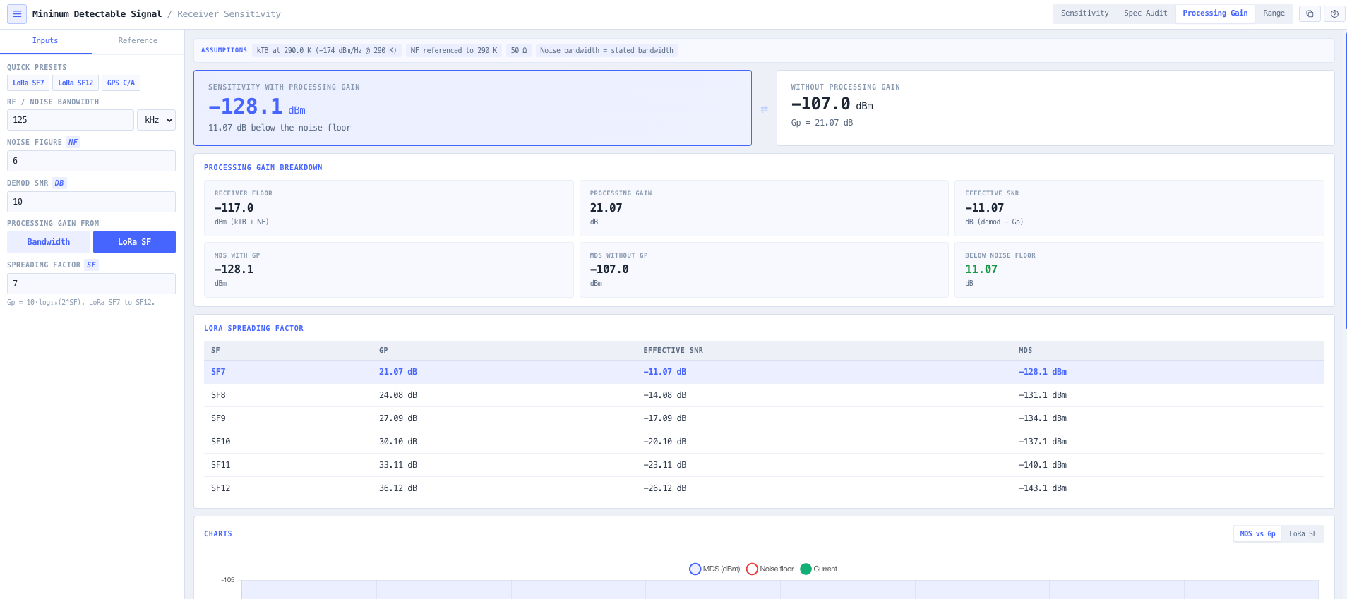
A spread spectrum waveform occupies far more bandwidth than its information rate, and the receiver recovers a processing gain Gp = 10·log₁₀(BW ÷ R). That gain lowers the effective required SNR, so the sensitivity drops by Gp and can sit tens of dB below the thermal noise floor, exactly as a GPS or LoRa receiver does. A LoRa spreading factor table reports SF7 to SF12.

Detection margin and maximum range

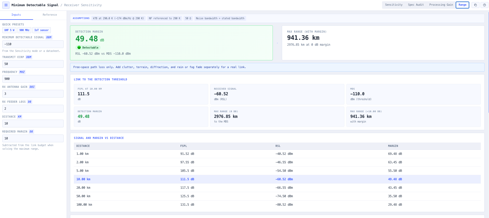
Build the received signal from the EIRP, free space path loss, receive antenna gain, and feeder loss, and compare it against the MDS for a colour coded detection margin. The maximum range is solved from the path loss the link can tolerate before the signal reaches the threshold, with and without a required margin.

Free space stated explicitly

The range figures use free space path loss alone. Real paths lose more to clutter, terrain, diffraction, and fade, so the free space range is an optimistic upper bound. The tool states this plainly and leaves the excess loss and fade margin to be added knowingly rather than buried in a single number.

Browser only computation

Runs entirely in your browser. No bandwidths, sensitivities, or link parameters are submitted to a server. Useful for commercially confidential work, classified projects, or any environment where information security policy prohibits sending engineering data to third party services.

Standards & methodology

  • Thermal noise density −174 dBm/Hz defined as kT at the 290 K reference temperature
  • Noise figure referenced to 290 K, added directly to the kTB thermal floor
  • Processing gain defined as Gp = 10·log₁₀(occupied bandwidth ÷ information rate)
  • Antenna factor AF = 20·log₁₀(f_MHz) − G_dBi − 29.79 for a 50 Ω system
  • Free space path loss = 32.44 + 20·log₁₀(d_km) + 20·log₁₀(f_MHz)

When to use this tool

  • Computing the minimum detectable signal of a receiver from its bandwidth, noise figure, and required SNR
  • Expressing a receiver sensitivity as a voltage to dial into a signal generator on the bench
  • Turning a sensitivity into a minimum detectable field strength for a monitoring or EMC survey
  • Reverse solving a datasheet sensitivity into the noise figure and SNR budget it implies
  • Sanity checking whether a quoted sensitivity is physically possible for its stated bandwidth
  • Comparing competing radio sensitivities on a like for like bandwidth basis
  • Sizing the processing gain a spread spectrum waveform needs to reach a target sensitivity
  • Estimating the sensitivity of a LoRa link at a given spreading factor
  • Checking why a GPS or DSSS receiver works with the signal below the thermal noise floor
  • Computing the detection margin of a received signal against the receiver threshold
  • Estimating the maximum free space range at which a signal reaches the minimum detectable level
  • Teaching receiver sensitivity and the noise floor with live, interactive results

Is this the right tool for you?

Reach for the Minimum Detectable Signal Calculator in any of the following situations.

  • You are specifying a narrowband radio and need the minimum detectable signal at 12.5 kHz for a 6 dB noise figure and a 12 dB required SNR.
  • You have a datasheet that quotes −119 dBm sensitivity but does not state the assumed SNR, and you want the noise figure and SNR budget the number implies.
  • You are comparing two handheld radios whose sensitivities are quoted at different bandwidths and need them on a like for like basis.
  • You are checking whether a vendor claim of −125 dBm at 25 kHz is physically possible or below the thermal floor.
  • You are planning a LoRa deployment and need the sensitivity at SF7 through SF12 to work out the link budget at each data rate.
  • You are explaining to a client why a GPS receiver works with the signal tens of dB below the thermal noise floor.
  • You are running a spectrum monitoring survey and need the minimum detectable field strength in dBµV/m for your receiver and antenna.
  • You are setting up a signal generator on the bench and need the receiver sensitivity as a voltage rather than a power.
  • You are sizing a 900 MHz telemetry link and need the detection margin at 10 km and the maximum range before the signal reaches the threshold.
  • You are budgeting a low power IoT sensor link and need the free space range at 14 dBm EIRP against a −137 dBm sensitivity.
  • You are auditing a receiver chain and want to see how the noise figure and required SNR each move the sensitivity.
  • You are operating under a security regime that prohibits sending design data to third party services and need a calculator that runs entirely in your browser.

Frequently asked questions

How do I calculate the minimum detectable signal?

Add the thermal noise floor, the receiver noise figure, and the required SNR. MDS equals −174 dBm/Hz plus 10·log₁₀ of the bandwidth in Hz, plus the noise figure in dB, plus the required SNR in dB. For a 12.5 kHz channel with a 6 dB noise figure needing 12 dB of SNR, the thermal floor is −174 + 41 = −133 dBm, the receiver floor is −127 dBm, and the MDS is −115 dBm. The calculator does this live and also expresses the result as a voltage and a field strength.

What is the difference between the noise floor and the minimum detectable signal?

The noise floor is the noise power at the receiver input, kTB plus the noise figure. The minimum detectable signal is the noise floor plus the SNR the demodulator needs to actually recover the signal. So the MDS is always above the noise floor by the required SNR. A signal exactly at the noise floor has a 0 dB SNR, which is the classic definition of the minimum detectable signal for a simple energy detector, but a real demodulator needs several dB more, and that margin is the required SNR term.

Why does a wider bandwidth raise the minimum detectable signal?

Because thermal noise is spread evenly across frequency, so a wider channel collects more of it. The noise power rises as 10·log₁₀ of the bandwidth, which is 3 dB for every doubling. A 25 kHz channel has a 3 dB higher floor than a 12.5 kHz channel and therefore a 3 dB worse sensitivity, all else equal. This is why narrowband systems are more sensitive and why reducing the receiver bandwidth to match the signal improves the minimum detectable level.

How can a GPS or LoRa receiver detect a signal below the noise floor?

Through processing gain. A spread spectrum waveform occupies far more bandwidth than its information rate, and the receiver correlator concentrates the signal energy while averaging the noise, recovering a processing gain of 10·log₁₀ of the bandwidth divided by the information rate. That gain is subtracted from the demodulator SNR to give the effective SNR needed at the input, so the sensitivity drops by the processing gain and can sit tens of dB below the thermal noise floor. A GPS C/A signal spreads 50 bit/s across about 2 MHz for roughly 46 dB of gain, which is why it works far under the noise.

How do I check whether a datasheet sensitivity is realistic?

Compare it against the thermal floor for its bandwidth. The gap between the quoted sensitivity and the thermal floor is the sum of the noise figure and the required SNR, so it should be a positive number of a sensible size, typically 10 to 25 dB. If the quoted sensitivity is below the thermal floor for the stated bandwidth, it is physically impossible and the bandwidth or the figure has been misread. The Spec Audit mode does this automatically, flags the impossible case, and splits the budget into the implied noise figure and SNR.

What required SNR should I use?

It depends on the modulation and the target error rate. A simple detection threshold is 0 dB, analog SSB or AM voice needs about 10 dB, analog FM to 12 dB SINAD needs about 12 dB, digital voice like P25 or DMR reaches its reference error rate around 5 dB, QPSK needs about 10 dB, and 64-QAM needs around 22 dB. The Reference tab lists these as indicative ranges for orientation. They are not a specification, and the real figure is whatever the demodulator in your radio needs for the error rate you are designing to.

Does the range calculation include terrain and clutter?

No. The range figures use free space path loss alone, so they are an optimistic upper bound rather than a prediction. Real paths lose more to clutter, terrain, diffraction, building penetration, and rain or fog fade, and gain nothing back. The tool states the free space assumption explicitly and leaves the excess path loss and the fade margin to be added separately, so you can see the free space bound and then apply the site specific losses knowingly. For a full propagation prediction use a path loss or coverage tool.

Does any data leave my browser?

No. The calculator runs entirely in your browser. No bandwidths, sensitivities, or link parameters are submitted to a server. Useful for commercially confidential work, classified projects, or environments where information security policy prohibits sending engineering data to third party services.