Bring your own mine — import, draw, or start from the demo
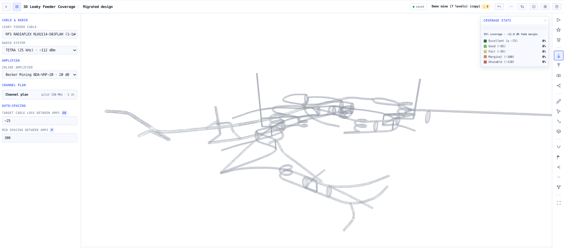
Import a real mine’s centreline geometry through a validating wizard: 3D DXF strings (LINE / LWPOLYLINE / POLYLINE-VERTEX as Surpac, Vulcan, Deswik, and Micromine export, with $INSUNITS detection and a per-layer mapping step assigning drift types, no-cable flags, and stope roles), waypoint CSV with header auto-detection, KML and GeoJSON LineStrings (altitudes used when present), and the native noim3-mine JSON. The pipeline welds junctions to the router tolerance, inserts tees, re-orients and splits drifts so the cable cascade always runs the right way, derives the level table, checks connectivity and loops, and recentres survey-grid coordinates — and shows the full report before anything is accepted. After import, draw drifts on a level plane with waypoint snapping, drag/insert/delete waypoints, edit per-drift properties, generate spiral and straight declines, vertical raises, shafts, and ore passes between levels, and place stopes by dragged footprint — all with undo. Or start from the built-in immutable seven-level demo mine (editing it forks a library copy).
Design the cable — auto-route or draw your own runs and splitters
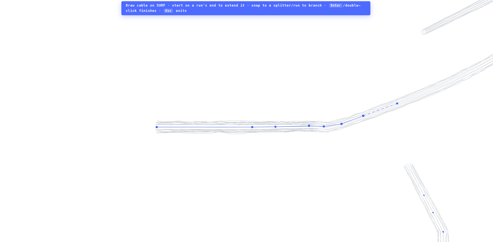
The radiating cable auto-routes through the primary access drift, the conveyor decline, and each level main on placement, respecting the level connections and the no-cable annotations on raises, ore passes, ventilation shafts, and production stopes. Or switch to manual (blank-canvas) mode and lay the cable yourself: Draw cable clicks waypoints along the runs (start on an existing run’s endpoint to extend it), Set start (headend) marks where the feed / base station connects, and Place splitter drops a power splitter — 2-way by default, set 2/3/4-way — that breaks the run into input and branch segments so the 10·log10(N) + insertion loss is actually applied downstream. Draw branch runs snapped to the splitter to add outputs; drawn cable snaps to splitters and amps; per-section delete, per-splitter removal, and clear-all keep it tidy. A Cable network inspector lists every routed segment, splitter, and unconnected drift, and the drawn cable drives the coverage directly.
Channel plan, AGC pilot, and the voice carrier
Coverage runs off a duplex channel plan, not a single frequency. The plan carries a downlink-only +0 dBm AGC pilot plus your traffic channels — each a downlink and an uplink carrier — and coverage is evaluated on the worst (highest-frequency) channel per direction, shown in the Eval @ chip, so a VHF voice channel and a UHF data channel show their different coverage. The AGC holds the pilot flat and restores it at every amplifier, while the traffic carriers ride a back-off below it (default −7 dB, editable per channel to protect amplifier headroom). The heatmap, the per-tier statistics, and the off-air hover levels are all the voice carrier — the level a worker actually talks on — while the pilot is reported separately as the AGC reference. The same plan feeds a composite-power and intermodulation read-out for amplifier-overload checks.
Live ITU-R stub physics — P.526 UTD corner diffraction and P.1238 corridor decay
Non-cabled drifts (stope access stubs, dead ends, ore-zone crosscuts) get their coverage from corner diffraction computed live at the channel-plan frequency. Per junction, the engine extracts the actual corner geometry from the drift waypoint headings and evaluates the ITU-R P.526-16 §6 UTD wedge-diffraction kernel with hard-rock material defaults, power-summing both diffracting corners at T-junctions and four-way intersections. Propagation along the stub past the corner follows the ITU-R P.1238-13 §3.1 corridor log-distance model, switching from the line-of-sight to the non-line-of-sight coefficient set past an internal bend. Both models are under unit test against the recommendations.
Floor-level voice-coverage heatmap — cascade, coupling, and body loss
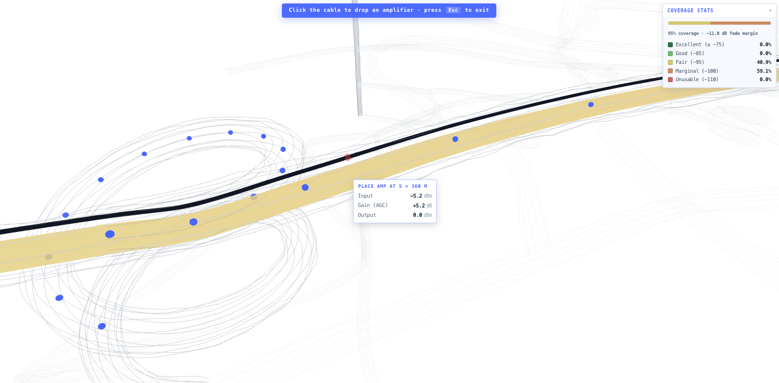
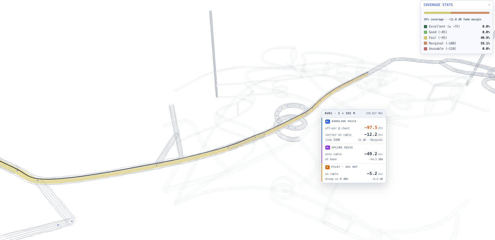
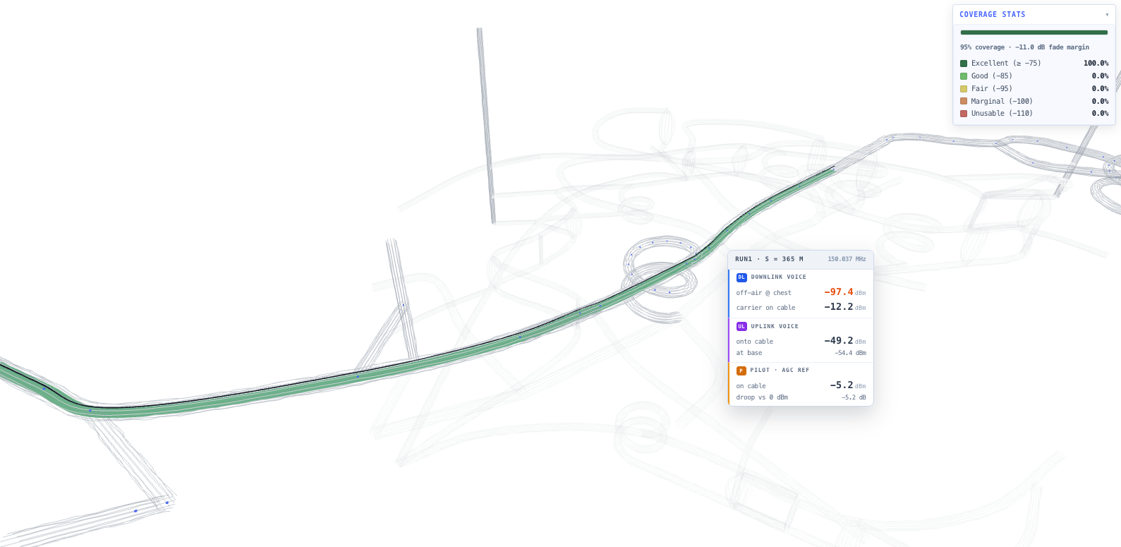
Coverage renders as a heatmap ribbon along every drift floor at the worst-case receiver position. On cabled drifts each station combines the along-cable cascade (per-100 m loss times the cable run distance, through every splitter and amplifier) with the cable’s measured radial coupling loss from the ceiling-mounted cable to the chest-height receiver, the operator body loss, and the traffic-carrier back-off — then classifies it at the chosen reliability percentile. On non-cabled drifts the ribbon is diffraction-fed from every junction shared with a cabled drift. It is a true per-drift picture that captures the level-by-level loss accumulation, the splitter dilution, and the stub shadowing a single-run 2D cascade cannot show.
Downlink, uplink, and worst-of-link coverage modes
Downlink mode renders the voice level a handheld hears at the worst-case floor position — for gap identification and amplifier-spacing decisions. Uplink mode renders the level reaching the first upstream amplifier from a portable transmitting at each point — the limiting factor for talk-back, with the full budget to the headend and the cascaded uplink noise figure carried in the hover. Worst-of-link renders the minimum of the two, the single honest "can a worker use the radio here" view that finds holes where a worker can hear the base station but cannot reach it back. Diffraction-fed stubs carry no cable to inject into, so uplink and worst-of-link cover cabled drifts only — the statistics card discloses it.
Level slicing, reliability percentile, and the three-level hover
The level slice selector in the status bar (Off, L1 through L7) restricts the heatmap to one level’s band and dims the geometry above and below, so each level reads without overdraw — the way you find the worst-case run per level. The reliability percentile in Design settings (50 % median, 90 %, 95 % design-of-record, 99 % critical) applies the lognormal shadow-fading margin, with the cable’s cl50→cl95 coupling-loss spread setting the σ so 95 % reproduces cl95 with no double count. Hover any heat point for the three levels — DL voice (off-air at chest and on the cable), UL voice (injected back onto the cable and the level at base), and the pilot (the AGC reference and its droop) — or hover an amplifier marker for its input, AGC gain, output, and saturation state. The coverage statistics overlay doubles as the legend with live per-tier percentages, and splitter labels toggle on for an installation-document review.
Cable library fitted to manufacturer datasheets
A datasheet-fitted radiating-cable library: RFS RADIAFLEX (RLK114 VHF and the RLKU broadband series) and ZCG / Benelec 1/2" corrugated 50 Ω cables, plus DD-LFC-350, RNG-350, and Rojone CC-3529 75 Ω VHF/UHF cables. Each carries an along-cable loss curve as a least-squares K₁·√f + K₂·f fit against the manufacturer datasheet tables plus the per-cable cl50 / cl95 radial coupling-loss curve at the reference distance — with provenance recorded and any estimated field flagged. The channel-plan frequency drives the cable loss, the coupling loss, the UTD corner diffraction, and the corridor decay together, and the radio system selector (analogue FM, P25, DMR, TETRA, NXDN, LTE MC) sets the tier thresholds from the ITU-R M.1808 reference sensitivities.
Mine library, self-contained project files, and autosave
Mines live in a named browser-storage library alongside the built-in demo — select, rename, duplicate, delete, and export to a .mine.json file. Projects autosave to local storage, and a project exports to a self-contained .lf3d.json from the Projects picker — cable, channel plan, radio system, amplifiers, your drawn cable runs and splitters, and the full mine geometry embedded, so a shared file re-imports later without the original mine.
Honest Beta scope
The tool is in Beta and says so. The RF maths is under unit test against the ITU-R recommendations — including operator body loss and the traffic-carrier back-off — but the model has stated limits: the cable model is a tree, so loops in the drift network are cabled along the first-found path (disclosed per junction — mark a redundant leg no-cable to choose explicitly); DXF arcs, splines, and block inserts are skipped with a disclosed count; coupling loss above a cable’s characterised band clamps; and the engine does not yet model frequency-dependent cable bend loss, full vendor splitter/tap insertion loss, polarisation, or the leakage-vs-radiating-mode regime. For the 2D installation cascade with full vendor splitter and tap data and a bill of materials, use the 2D Leaky Feeder Designer.