Microwave Link Planning

Log Distance Path Loss Calculator

Empirical path loss with environment specific exponents and log normal shadow fading. Compute received power, maximum range, and link availability for cellular, private LTE, WiFi, IoT, indoor DAS, tactical VHF and UHF, and warehouse and factory deployments.

Overview

Free space path loss is the right model for satellite links above the atmosphere and short range line of sight links. It is the wrong model for almost everything else. Real terrestrial deployments cover urban canyons, suburban streets, dense city cores, office buildings, warehouses, factories, and forested countryside, where path loss does not scale with the inverse square of distance. Diffraction over buildings, reflection off the ground, multipath fading, foliage absorption, and the basic geometry of a transmitter and receiver embedded in a built environment all add to the loss. The result is path loss that scales with the inverse of distance to a power n greater than 2, where n is environment specific and called the path loss exponent.

The noIM₃ Log Distance Path Loss Calculator implements the empirical model PL(d) equals PL(d0) plus 10 n log of d over d0 plus X sigma, where PL(d0) is the reference path loss at a calibration distance, n is the environment specific path loss exponent, and X sigma is a zero mean log normal random variable representing shadow fading. The reference path loss is auto derived from free space at the calibration distance (typically 1 m for indoor or 100 m or 1 km for outdoor) or can be overridden with a measured value for sites with drive test or walk test calibration data.

Built in environment presets cover the full range of practical deployments. Free space (n equals 2.0). Urban macro (n equals 3.0 to 3.5). Suburban (n equals 2.7 to 3.0). Dense urban obstructed (n equals 4 to 5). Indoor office line of sight (n equals 1.6 to 1.8, where waveguiding effects in corridors actually beat free space). Indoor non line of sight (n equals 3 to 4). Factory line of sight (n equals 1.6 to 2.0). Factory obstructed (n equals 2 to 3). In home residential (n equals 3.0). Each preset ships with a typical shadow fading standard deviation (3 to 12 dB) for realistic link availability planning.

Capabilities

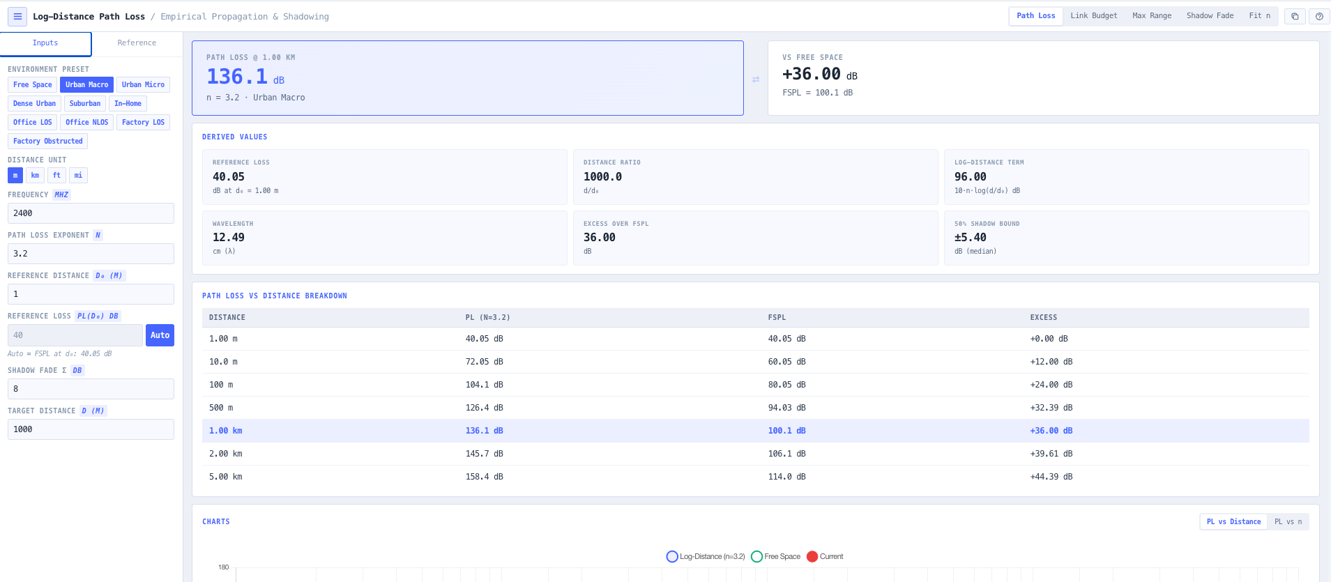
Log distance path loss model

Implements PL(d) equals PL(d0) plus 10 n log of d over d0. Reference path loss PL(d0) at the calibration distance is auto derived from free space (PL(d0) equals 20 log d0 plus 20 log f minus 27.55 for d0 in metres and f in MHz) or overridden with a measured value for calibrated models. Path loss output in dB ready for direct subtraction in the link budget.

Environment preset library

Nine plus environment presets covering free space, urban macro, urban micro, suburban, dense urban obstructed, indoor office line of sight, indoor non line of sight, factory line of sight, factory obstructed, and in home residential. Each preset sets the path loss exponent n and the shadow fading standard deviation sigma to industry typical values, with manual override for site specific calibration.

Reference distance calibration

Calibration distance d0 selectable to match the deployment scale (1 m for indoor and short range, 100 m for typical outdoor cellular, 1 km for macro cellular). Reference path loss at d0 auto computed from free space, with manual override for sites that have a measured calibration point from drive test or walk test data.
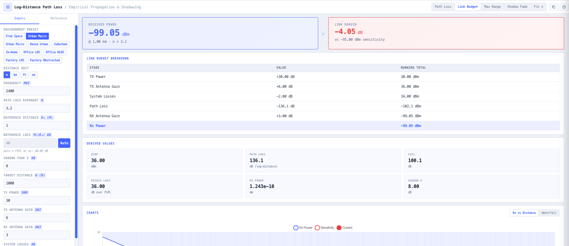
Full link budget

Applies the path loss to the full RF chain. Transmit power, transmit antenna gain, transmit feeder and connector loss, path loss, receive antenna gain, receive feeder loss, all combined to deliver received signal level in dBm and link margin against a configured receiver sensitivity. EIRP also surfaced for licence compliance cross check.

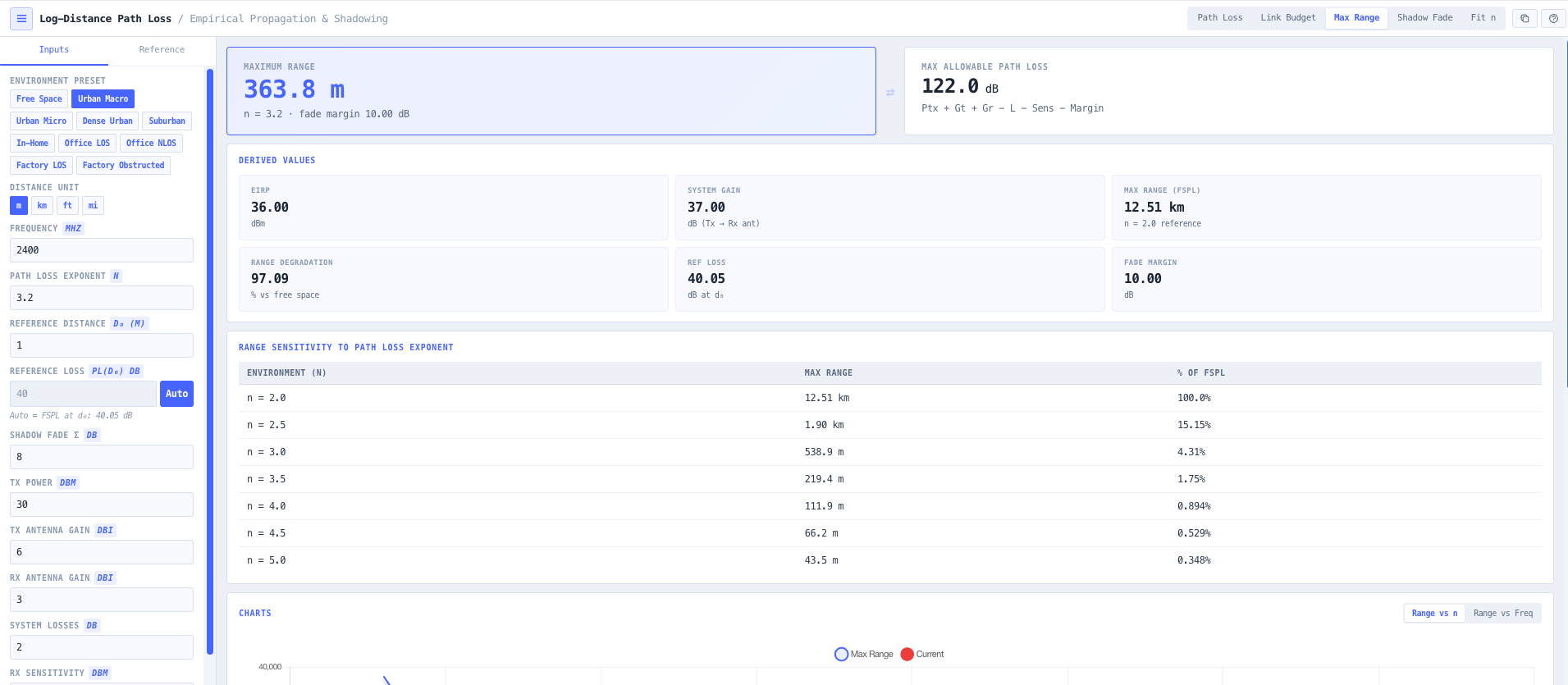
Maximum range solver

Inverts the log distance equation to solve for the maximum link distance achievable at a target maximum allowable path loss (MAPL) or against a configured receiver sensitivity. Useful for cell radius estimation, coverage planning for indoor DAS, and sensitivity limited IoT and LoRa deployments where the design question is how far can the link reach.

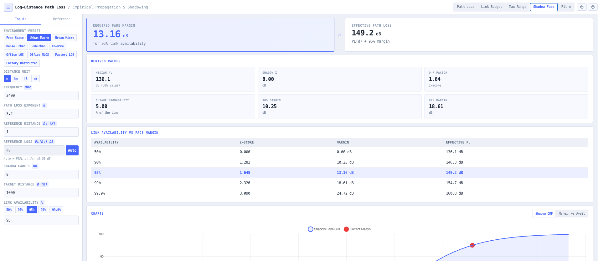
Log normal shadow fading

Models large scale shadow fading as a zero mean log normal random variable X sigma with environment typical standard deviation (3 to 12 dB). Computes the fade margin required for a target link availability (50, 90, 95, 99, 99.9 per cent) using the inverse Q function. Reliability driven link design rather than mean path estimation alone.

Maximum allowable path loss (MAPL) workflow

Configure the receiver sensitivity, fade margin, and antenna gains, and the calculator returns the MAPL the link can survive. Combined with environment preset and frequency, this directly translates to a coverage radius for cell planning. Useful for cellular and private LTE coverage planning, IoT gateway placement, and DAS antenna density sizing.

Interactive visualisation

Charts cover path loss versus distance on a log scale, received power versus distance, path loss exponent sensitivity (showing how the n value drives the slope), and shadow fading cumulative distribution function for the configured availability target. Useful for design intuition and producing visuals for engineering reports and customer presentations.

Browser only computation

Runs entirely in your browser. No transmit power, antenna gain, environment, or coverage data is submitted to a server. Useful for commercially confidential cellular and IoT infrastructure planning and environments where information security policy prohibits sending engineering data to third party services.

Standards & methodology

  • Empirical log distance path loss model (Rappaport, Wireless Communications: Principles and Practice)
  • ITU R P.1411. Propagation data and methods for short range outdoor links
  • ITU R P.1238. Propagation data and methods for indoor radio systems
  • 3GPP TR 38.901. Study on channel model for frequencies from 0.5 to 100 GHz
  • IEEE 802.15.3a indoor channel model reference (path loss exponents and shadow fading)

When to use this tool

  • Cell radius and coverage estimation for private LTE and 5G deployments
  • Indoor DAS and WiFi coverage prediction in offices, warehouses, and large indoor spaces
  • LoRa and IoT link budget analysis with path loss exponent tuning against deployment environment
  • Tactical VHF and UHF range prediction in urban, suburban, and rural terrain
  • Link availability and fade margin design under log normal shadowing
  • Calibration of empirical propagation models against drive test or walk test data
  • Educational demonstrations of path loss scaling versus frequency and distance
  • Sizing antenna gain and transmit power against a target coverage radius
  • Comparing two candidate sites or environments for the same coverage target
  • Producing coverage estimates for cellular small cell, private LTE, and 5G NR FR1 deployments
  • Sanity checking vendor coverage claims against the underlying environment exponent
  • Sizing IoT gateway placement for sensor networks across distributed sites

Is this the right tool for you?

Reach for the Log Distance Path Loss Calculator in any of the following situations.

  • You are sizing the cell radius for a private LTE deployment on a mine site, port, or factory and need realistic path loss against the actual environment exponent rather than free space.
  • You are designing indoor DAS coverage for an office building, hospital, or warehouse and need to choose path loss exponents that reflect line of sight corridors and obstructed back of house.
  • You are deploying a LoRa or IoT sensor network and need to confirm that the gateway can reach the most distant sensor against the deployment environment exponent and receiver sensitivity.
  • You are estimating tactical VHF or UHF radio range across urban, suburban, or rural terrain and need empirical environment specific propagation rather than free space.
  • You are responsible for a private 5G NR FR1 deployment and need coverage estimation against industrial environment exponents (factory, refinery, dense urban infill).
  • You are calibrating a propagation model against drive test or walk test data and need to override the reference path loss at the calibration distance with measured values.
  • You are planning a high availability link (99.9 per cent) and need to compute the fade margin required to absorb log normal shadow fading at the configured environment standard deviation.
  • You are comparing two candidate cell sites for the same coverage target and want a side by side coverage radius estimate against the environment exponent at each site.
  • You are evaluating whether to use a higher gain antenna or a higher transmit power to extend coverage in a particular environment.
  • You are sanity checking a vendor proposed cell radius claim against the underlying environment exponent and receiver sensitivity.
  • You are sizing antenna density for an indoor DAS system across a multi storey building and need maximum range estimation per antenna against the indoor environment exponent.
  • You are training new RF engineers in environment specific path loss and want a teaching tool that shows how the exponent n drives the slope of the path loss versus distance curve.
  • You are deploying a private LTE network over a large industrial site and need to choose between free space, suburban, and dense urban exponents based on the actual obstruction environment.
  • You are responsible for coverage planning across regional and remote Australian deployments where terrain and vegetation drive the exponent selection.
  • You are operating under a security regime that prohibits sending coverage planning data to third party services and need a calculator that runs entirely in your browser.

Frequently asked questions

What is the log distance path loss model?

PL(d) equals PL(d0) plus 10 n log base 10 of (d divided by d0), where PL(d0) is the path loss at a reference distance d0, n is the path loss exponent, and d is the distance of interest. With shadow fading, an additional log normal random variable X sigma is added. The model is empirical, calibrated by drive test or walk test data, and is the standard approach for terrestrial coverage planning where free space path loss is too optimistic.

What path loss exponents should I use for which environments?

Free space n equals 2.0 (satellite or short line of sight). Urban macro n equals 3.0 to 3.5. Suburban n equals 2.7 to 3.0. Dense urban obstructed n equals 4 to 5. Indoor office line of sight n equals 1.6 to 1.8 (corridors waveguide and beat free space). Indoor non line of sight n equals 3 to 4. Factory line of sight n equals 1.6 to 2.0. Factory obstructed n equals 2 to 3. In home residential n equals 3.0. The calculator includes presets that set both n and the shadow fading sigma to industry typical values.

How is reference distance d0 chosen?

Match the deployment scale. Indoor and short range systems typically use d0 equals 1 m. Outdoor cellular small cells typically use d0 equals 100 m. Macro cellular networks typically use d0 equals 1 km. Reference path loss PL(d0) is then computed from free space at the chosen d0 (or overridden manually with a calibrated value). The choice of d0 does not change the path loss at any d greater than d0, but it does determine where the model anchors and how sensitive it is to errors in PL(d0).

How does shadow fading affect the design?

Shadow fading is a slowly varying random variation in path loss caused by large scale obstruction (buildings, terrain, foliage) that an environment averaged exponent cannot represent. It is modelled as a zero mean log normal random variable X sigma with standard deviation sigma typically 3 to 12 dB depending on environment. To meet a target availability (for example 90 or 99 or 99.9 per cent) at the cell edge, an additional fade margin must be added to the budget, sized using the inverse Q function. The calculator computes this margin automatically against the configured availability target.

How is this different from FSPL and Friis?

Free Space Path Loss and Friis assume ideal line of sight propagation in vacuum, with path loss scaling as 20 log d (n equals 2). The log distance model extends this to terrestrial environments where path loss scales as 10 n log d with n typically 2 to 5 depending on environment. Use FSPL or Friis for satellite and short line of sight links. Use the log distance model for everything else. Use the noIM₃ Link Planner for full ITU P.530 microwave link design with terrain and atmospheric effects.

What does the maximum range solver do?

Inverts the log distance equation to compute the maximum distance d max at which the path loss equals the configured maximum allowable path loss (MAPL) or causes the received power to drop to the receiver sensitivity. Useful for cell radius estimation in coverage planning, indoor DAS antenna spacing, and sensitivity limited IoT and LoRa deployments. The MAPL form is convenient for cellular planning where the link budget is typically fixed and the question is how far the cell reaches.

How do I calibrate the model against measured data?

Drive or walk test the deployment at a reference distance d0, measure the path loss PL(d0), and override the auto computed free space value with the measured one. The Fit n mode then derives the path loss exponent n implied by a single measured (distance, path loss) point, given d0 and PL(d0). For a more robust fit over many measurements at different distances, run several points through Fit n and average the result, or fit n by least squares externally. Calibrated models routinely deliver sub 5 dB rms error against measurement, compared to 10 to 20 dB error from generic free space estimates in obstructed environments.

Does any data leave my browser?

No. The calculator runs entirely in your browser. No transmit power, antenna gain, environment, or coverage data is submitted to a server. Useful for commercially confidential cellular and IoT infrastructure planning and environments where information security policy prohibits sending engineering data to third party services.