Compose multi tone signals, apply window functions, and measure THD, SFDR, SNR, SINAD, and ENOB. A complete frequency domain analysis workbench for RF and digital signal processing engineers running entirely in your browser.
Free on a Standard account, with no time limit. No credit card.
FFT Spectrum Analyser
10 inputs→13 outputs
Walkthrough
See it working
FFT Spectrum Analyser1 / 3
Overview
What the FFT Spectrum Analyser does
A spectrum analyser is the most useful instrument in any RF or digital signal processing toolbox. It tells you what frequencies are present, what their amplitudes are, and how cleanly the signal is generated. The trouble with hardware spectrum analysers is that they are expensive, fixed at a particular sample rate, and not always available when you need them. Software analysers based on the Fast Fourier Transform deliver the same view, often with more flexibility (any sample rate, any signal composition, any window function), and are particularly useful for teaching, ADC characterisation, RF system simulation, and verifying FFT implementations against known test vectors.
Read the full overview
The noIM₃ FFT Spectrum Analyser is a complete browser based frequency domain workbench. The signal composition stage builds composite signals from any number of components (sine, cosine, square, sawtooth, triangle, and DC), each with independent frequency, amplitude, and phase. Non sinusoidal waveforms are band limited via truncated Fourier series so harmonic aliases are avoided. Calibrated Gaussian AWGN noise can be injected at a configurable per bin dBFS floor. The synthesised signal is windowed and transformed via a Cooley Tukey radix 2 FFT supporting 64, 128, 256, 512, 1024, 2048, 4096, and 8192 points.
Seven window functions are implemented with the periodic (DFT even) convention required for FFT use. Rectangular, Hanning, Hamming, Blackman, Blackman Harris (4 term), Flat Top (5 term SRS), and Kaiser with beta equals 6. Each window is characterised by mainlobe width, peak sidelobe level, coherent gain (CG), and noise equivalent bandwidth (NEBW). Coherent gain correction is applied to the amplitude spectrum so single tone amplitude reads correctly across all window types. NEBW correction is applied to power spectral density. Spectral metrics (THD, SFDR, SNR, SINAD, ENOB) are computed from the corrected one sided spectrum with mainlobe aware harmonic detection that accounts for window broadened peaks.
Capabilities 9
Cooley Tukey radix 2 FFT
In place radix 2 decimation in time FFT supporting 64 to 8192 point lengths. Output is the one sided amplitude spectrum with frequency resolution of sample rate divided by FFT length. Coherent gain corrected so single tone amplitude reads correctly regardless of the window function applied.
Seven window functions
Rectangular (no windowing), Hanning, Hamming, Blackman, Blackman Harris (4 term), Flat Top (5 term SRS), and Kaiser (beta equals 6). Each implemented in periodic (DFT even) convention with live coherent gain and noise equivalent bandwidth (NEBW) correction. Window properties (mainlobe width, peak sidelobe level, CG, NEBW) are surfaced directly so the choice of window is informed.
Multi tone signal composition
Build composite signals from sine, cosine, square, sawtooth, triangle, and DC components, each with independent frequency, amplitude (0 to 1 full scale), and phase. Non sinusoidal waveforms are band limited via truncated Fourier series so harmonic aliases are avoided. Useful for ADC test signals, intermodulation test inputs, and arbitrary waveform synthesis.
Calibrated AWGN noise injection
Gaussian additive white noise at a configurable per bin dBFS floor. Calibrated against the FFT length so the noise level on the spectrum matches the configured value across all FFT sizes. Useful for SNR and ENOB measurement, sensitivity testing, and educational demonstrations of how noise floor scales with bandwidth and FFT length.
THD, SFDR, SNR, SINAD, ENOB
Total harmonic distortion computed as square root of sum of harmonic powers divided by fundamental, with plus or minus 2 bin peak search to capture window broadened peaks. SFDR is the difference between fundamental and the largest non harmonic spur. SNR and SINAD use summed noise bin power excluding fundamental and harmonic regions. ENOB equals (SINAD minus 1.76) divided by 6.02. All metrics derived from the coherent gain corrected one sided spectrum.
Three visualisation views
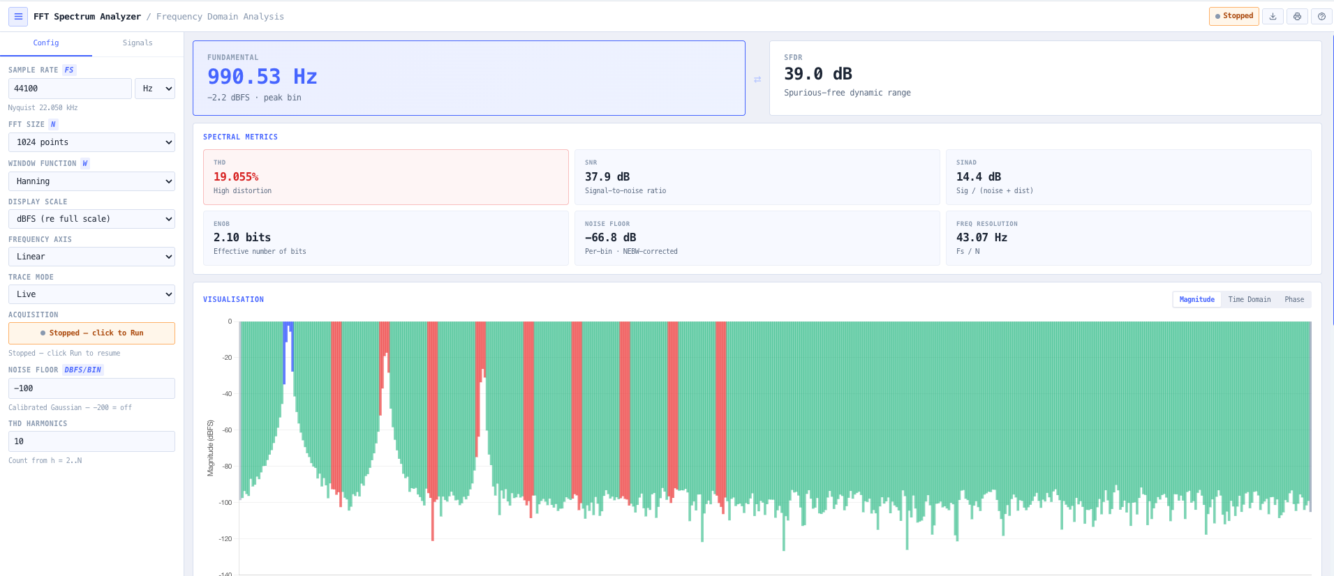
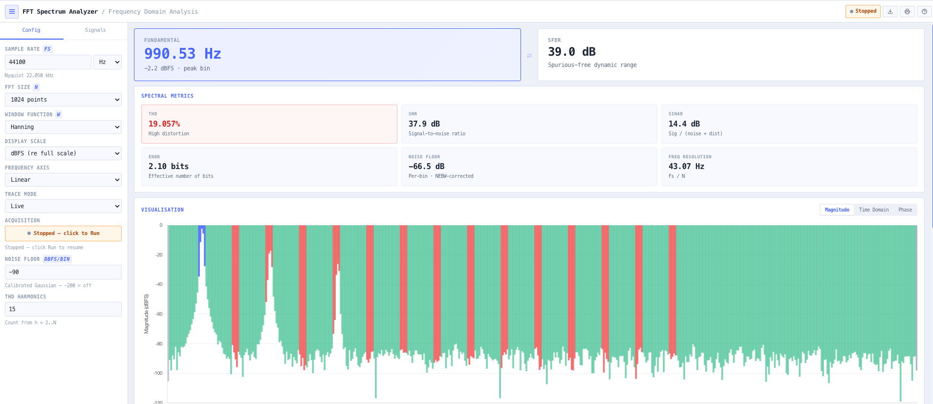
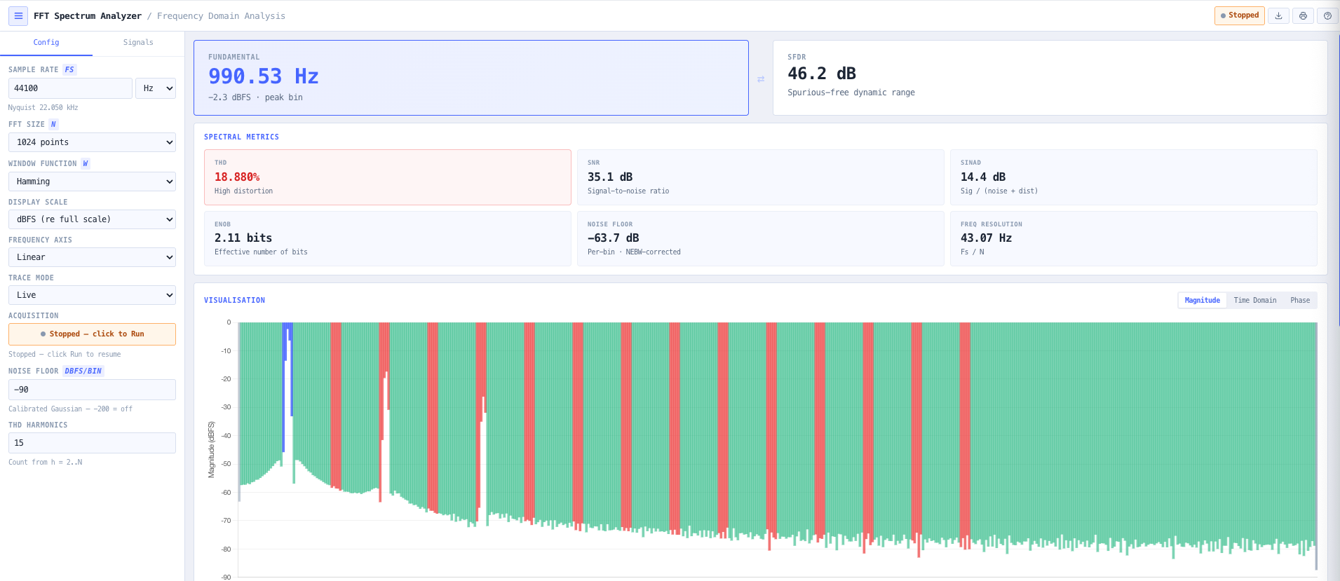
Magnitude spectrum bar chart with bins coloured by type (fundamental in blue, harmonics in red, spurs and noise in green). Time domain plot of the synthesised signal. Phase spectrum scatter of phase angle versus frequency for significant bins. Display scale switchable between dBFS, linear normalised, and power spectral density (full scale squared per Hz).
Trace modes and marker
Live trace updates as the signal composition changes. RMS average across N samples (N from 2 to 64) for noise floor smoothing. Peak hold for catching transient spurs. Movable marker reports exact frequency, magnitude, and delta against the fundamental at any selected bin. Linear or log frequency axis selectable.
CSV export and printable report
CSV export of every bin with frequency, magnitude, and phase. Printable text report covering signal composition, FFT parameters, window choice, and computed metrics. Suitable for measurement records, design documentation, and teaching exercise output.
Browser only computation
Runs entirely in your browser. No signal compositions, FFT data, or measurement results are submitted to a server. Useful for commercially confidential RF and DSP work, ADC characterisation under non disclosure, defence and intelligence signal analysis, and environments where information security policy prohibits sending engineering data to third party services.
Inputs and outputs
What goes in, what comes out
Inputs 10
Signal components (sine, cosine, square, sawtooth, triangle, DC) with frequency, amplitude (0 to 1 full scale), and phase per component
A Cooley Tukey radix 2 decimation in time FFT, in place, supporting power of two FFT lengths from 64 up to 8192 points. The output is a one sided amplitude spectrum with frequency resolution equal to sample rate divided by FFT length, coherent gain corrected against the active window function.
Why does the choice of window matter?
A real signal of finite duration has implicit discontinuities at the start and end of the FFT block, which spread spectral energy across many bins (spectral leakage). Window functions taper the signal smoothly to zero at the edges, reducing leakage at the cost of broader mainlobes. Different windows trade mainlobe width against sidelobe level differently. Rectangular has the narrowest mainlobe but worst sidelobes. Blackman Harris has very low sidelobes but a wide mainlobe. Flat Top has the flattest amplitude response across the bin (best for amplitude measurement) but is wide. Kaiser is parametric and tunable. The right choice depends on whether you are measuring amplitude, detecting spurs near a strong tone, or measuring noise floor.
What is coherent gain correction?
Every window has a coherent gain CG less than one (because the window tapers the signal). Without correction, single tone amplitude would read low by a factor of CG. The calculator applies CG correction to the amplitude spectrum so single tone amplitude reads correctly regardless of window choice. NEBW correction is also applied to power spectral density measurements so noise floor reads correctly.
How is THD calculated?
THD equals square root of the sum of harmonic powers divided by fundamental power, expressed as a percentage. Harmonics 2 through 9 are searched (or up to a configurable limit) using a plus or minus 2 bin peak search around the expected harmonic frequency to capture window broadened peaks. The result is reported in percentage and in dB so it can be cross checked against the ADC datasheet THD spec form.
What is ENOB and why does it matter?
Effective Number Of Bits is the equivalent resolution of an ideal ADC that would deliver the same SINAD as the real ADC under test. ENOB equals (SINAD minus 1.76) divided by 6.02. An 8 bit ADC with an ideal 49.92 dB SINAD has ENOB equals 8. Any harmonic distortion or noise above the quantisation floor reduces ENOB below the nominal bit count, so ENOB is a useful single number summary of overall ADC quality.
How is the noise floor calibrated?
Calibrated Gaussian additive white noise is injected at a configurable per bin dBFS level. The amplitude is scaled with FFT length so the per bin noise floor stays constant as you change FFT size, while the absolute integrated noise power scales correctly with bandwidth. This matches the way real ADC datasheets specify SNR and lets the analyser produce repeatable noise floor measurements regardless of the FFT length you choose.
How is this different from a hardware spectrum analyser?
A hardware spectrum analyser measures real signals from the world. The FFT Spectrum Analyser computes the spectrum of synthesised or imported signals. The mathematics is the same. Use the FFT Spectrum Analyser for synthesised test signal analysis, ADC characterisation against known inputs, teaching, and FFT verification. Use a hardware spectrum analyser when you need to measure a real RF signal off air or off a circuit board.
Does any data leave my browser?
No. The analyser runs entirely in your browser. No signal compositions, FFT data, or measurement results are submitted to a server. Useful for commercially confidential RF and DSP work, ADC characterisation under non disclosure, defence and intelligence signal analysis, and environments where information security policy prohibits sending engineering data to third party services.