RF Utilities

Noise Figure Calculator

Bidirectional Noise Figure to Noise Temperature conversion with cascaded receiver analysis using the Friis formula, system noise temperature with antenna and feed line contributions, and Y factor measurement support for low noise amplifier characterisation.

Overview

Noise figure is the gatekeeper of receiver sensitivity. The lower the noise figure, the lower the noise floor at the receiver input, and the more usable signal you can recover from a faint carrier. Every dB of noise figure improvement is a dB of free link margin in the budget. The trouble is that noise behaviour is expressed in two different vocabularies. Noise Figure in dB and Noise Temperature in Kelvin. They describe the same physical thing, but datasheets, receivers, and design tools mix them up. Cryogenic and satellite low noise amplifiers are usually quoted in Kelvin (5 K, 30 K, 70 K). Commercial receivers are usually quoted in dB (1 dB, 3 dB, 7 dB). Mixing the two without converting is a common source of design error.

The noIM₃ Noise Figure Calculator handles the conversion in both directions against a configurable reference temperature (typically 290 K). The standard relationships are implemented directly. T equals T0 times (10 to the power of NF over 10 minus 1). NF equals 10 log of (1 plus T over T0). Both forms are returned simultaneously alongside the linear noise factor F so the conversion is a glance rather than a separate calculation. Single component presets (Cryo LNA, Sat LNA, Good LNA, Avg RX, Basic RX) and an NF reference table spanning a cryogenic LNA through to a poor receiver accelerate component selection and rapid estimation.

Beyond conversion, the calculator computes cascaded system noise figure using the Friis formula. F equals F1 plus (F2 minus 1) over G1 plus (F3 minus 1) over (G1 G2) and so on across the receiver chain. This makes visible the design rule that the first amplifier in the chain dominates the system noise figure as long as its gain is high enough to suppress the noise contribution of subsequent stages. System noise temperature analysis adds antenna and feed line contributions for satellite and ground station work where antenna noise temperature is not negligible. Y factor measurement support lets you compute noise figure directly from hot and cold load measurements during LNA characterisation.

Capabilities

Bidirectional Noise Figure to Noise Temperature conversion

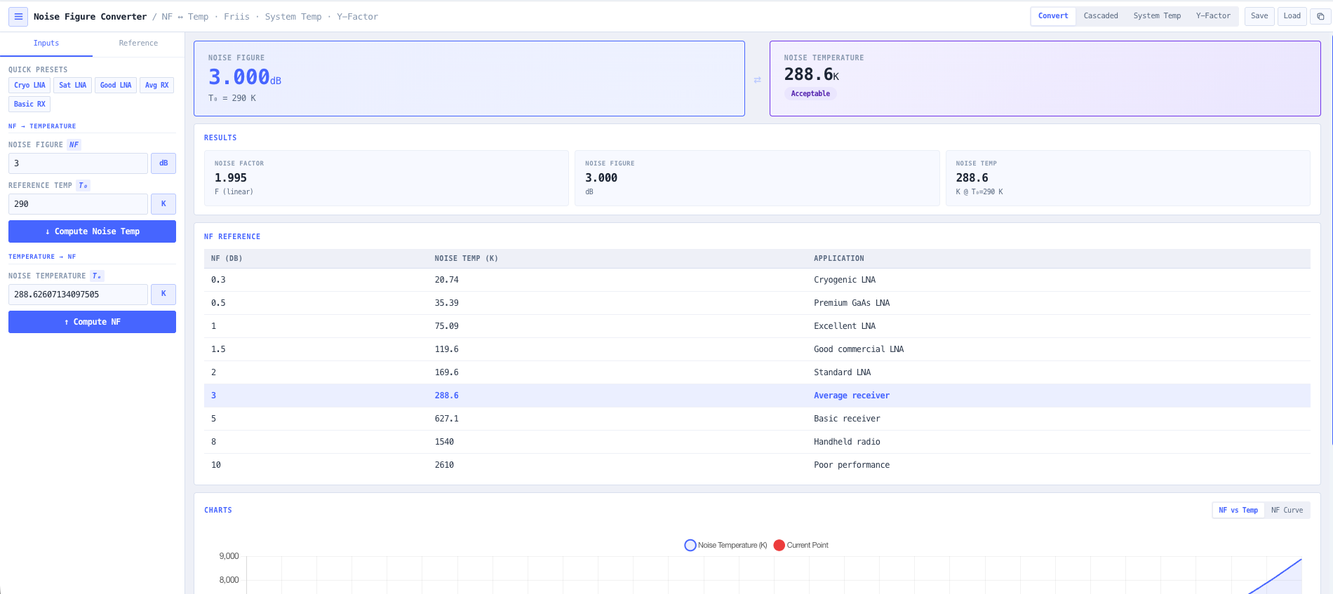
Standard conversion in both directions using T equals T0 times (10 to the power of NF over 10 minus 1) and NF equals 10 log of (1 plus T over T0). Reference temperature T0 is configurable (typically 290 K following IEEE convention). The linear noise factor F is surfaced alongside. All three quantities update simultaneously so the conversion is a read across, with an NF reference table and an NF versus noise temperature chart for context.

Cascaded noise analysis with the Friis formula

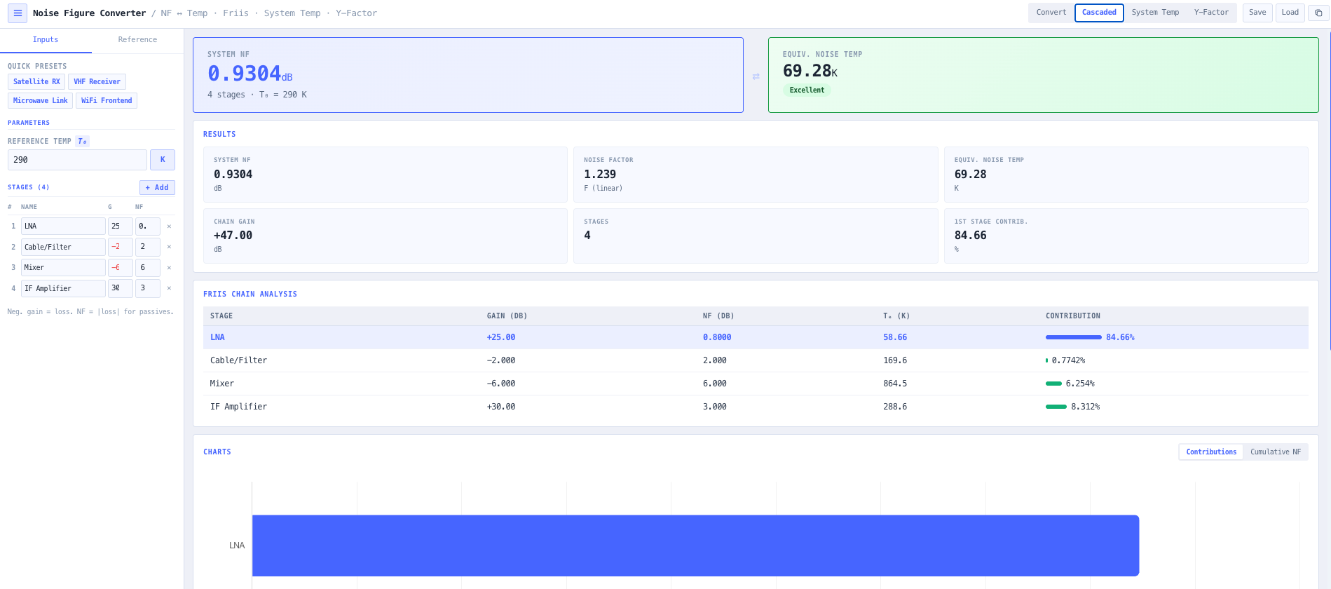
Compute the total system noise figure and noise temperature across multiple amplifier stages using the Friis formula. F equals F1 plus (F2 minus 1) over G1 plus (F3 minus 1) over (G1 times G2). Each stage accepts a name, a gain in dB (negative for a loss component such as a cable or waveguide), and a noise figure in dB. A per stage contribution table walks the chain so the dominant noise contributor is visible, alongside the cascaded NF, cascaded noise temperature, and total chain gain.

System noise temperature with antenna and feed line contributions

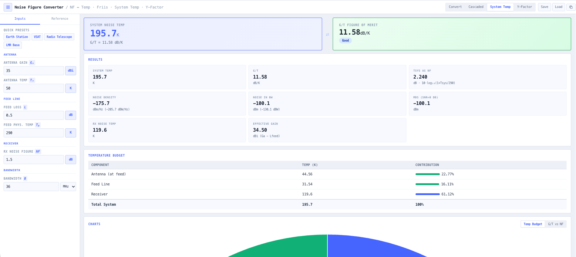
For satellite and ground station applications the system noise temperature combines the antenna, the feed line, and the receiver. T_sys equals Ta over Lc plus Tp times (1 minus 1 over Lc) plus T_receiver, referred to the receiver input, where Ta is the antenna noise temperature, Lc the linear feed loss, and Tp the feed physical temperature. The feed line both attenuates the incoming antenna noise and adds its own thermal noise. The G over T figure of merit, the noise power spectral density, the noise power in the configured bandwidth, and the minimum detectable signal are reported alongside.

Y factor measurement support

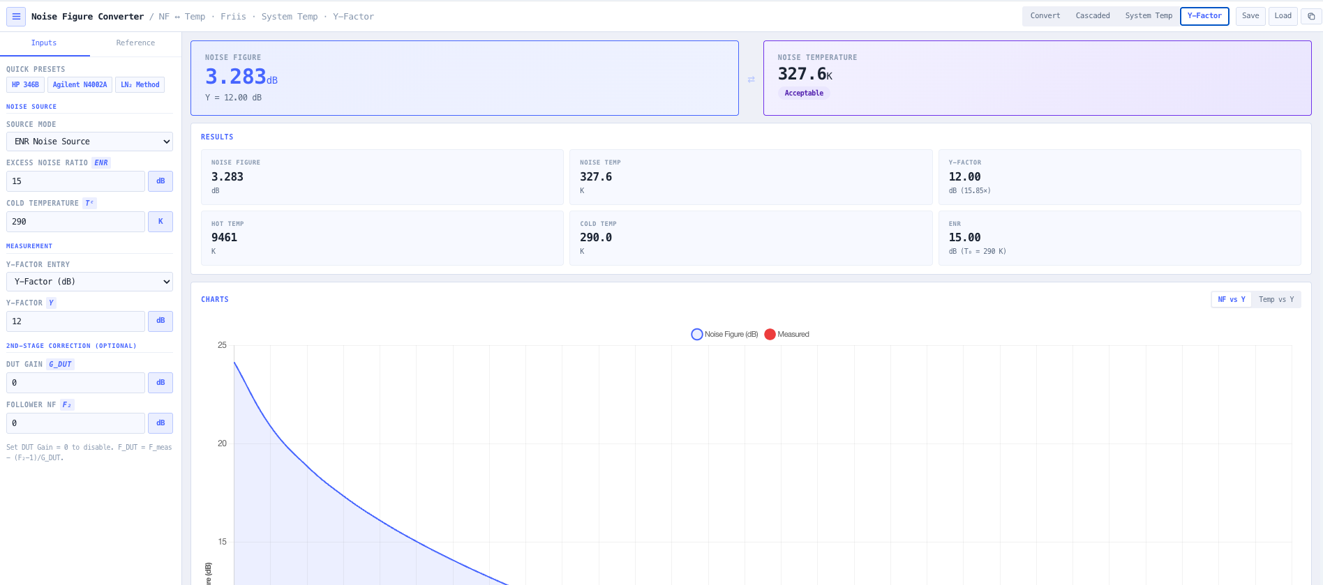
Compute noise figure directly from a Y factor measurement. The hot source is entered as an excess noise ratio (ENR) or a direct temperature, and the Y factor as dB, a linear ratio, or hot and cold power readings. The noise temperature follows from T_e equals (T_hot minus Y times T_cold) over (Y minus 1), then NF equals 10 log of (1 plus T_e over T0). An optional second stage correction removes the follower contribution: F_DUT equals F_measured minus (F2 minus 1) over G_DUT.

Single component and cascaded receiver presets

Single component presets seed typical noise figures for a cryogenic LNA (0.3 dB), a satellite LNA (0.8 dB), a good commercial LNA (1.5 dB), an average receiver (3.0 dB), and a basic receiver (6.0 dB). Cascaded presets seed full chains for a satellite receiver, a VHF receiver, a microwave link, and a WiFi frontend. System and Y factor modes carry their own presets (earth station, VSAT, radio telescope, LMR base, and calibrated noise sources). Useful for component selection and rapid estimation during design discussions.

Visualisation of NF versus noise temperature

Plots the relationship between Noise Figure in dB and Noise Temperature in Kelvin across the operating range, along with the cascaded stage contribution, the system temperature budget, and the Y factor relationships. Reinforces intuition for the non linear relationship at low noise figures, where small dB improvements translate to large temperature reductions, which is the design region for satellite and cryogenic work.

Browser only computation

Runs entirely in your browser. No noise figure values, gain stages, or system data is submitted to a server. Useful for commercially confidential receiver design work, satellite ground segment, defence and intelligence installations, and environments where information security policy prohibits sending engineering data to third party services.

Standards & methodology

  • IEEE definition of Noise Figure with reference temperature 290 K
  • Friis cascade noise factor formula
  • IEC 60050 international electrotechnical vocabulary noise definitions
  • Industry Y factor measurement methodology with calibrated noise sources

When to use this tool

  • Converting Noise Figure to Noise Temperature for satellite and cryogenic receiver design
  • Computing cascaded receiver noise figure across multiple amplifier stages with the Friis formula
  • Characterising low noise amplifiers via Y factor measurement during laboratory acceptance
  • Estimating system noise temperature for satellite ground stations including antenna and feed line contributions
  • Selecting low noise components for satellite, radio astronomy, and cryogenic systems
  • Identifying the dominant noise contributor in a multi stage receiver chain
  • Educational demonstrations of the noise figure and noise temperature relationship
  • Sanity checking vendor LNA specifications against expected system performance
  • Producing receiver noise budget evidence for satellite acceptance testing
  • Diagnosing receiver desensitisation by separating noise figure contribution from external interference
  • Auditing an inherited receiver design against current low noise component options
  • Designing radio astronomy receivers where every Kelvin of system noise temperature matters

Is this the right tool for you?

Reach for the Noise Figure Calculator in any of the following situations.

  • You are designing a satellite ground station receiver chain and need to compute system noise temperature including antenna noise, feed line loss, and the cascaded LNA and downconverter contributions.
  • You are converting a satellite or radio astronomy LNA datasheet that specifies 50 K noise temperature into Noise Figure in dB so you can compare it against a commercial receiver datasheet quoted in dB.
  • You are characterising a low noise amplifier in the laboratory using a Y factor measurement against a calibrated noise source and need to compute the noise figure from the measured Y factor and known excess noise ratio.
  • You are sizing a cascaded receiver chain and want to confirm that the front end LNA gain is high enough to suppress the noise contribution of the subsequent stages, identifying the dominant stage in the chain.
  • You are evaluating two candidate first stage LNAs (for example a 0.5 dB part versus a 0.3 dB part) and need to see how the dB difference translates to system noise temperature improvement and link margin.
  • You are designing a radio astronomy receiver where every Kelvin of system noise temperature improvement translates to longer integration baselines or weaker source detection thresholds.
  • You are producing receiver noise budget evidence for satellite acceptance testing and need a defensible cascaded noise figure or system noise temperature calculation.
  • You are diagnosing receiver desensitisation on a working network and want to separate the noise figure contribution of the receiver chain from external interference.
  • You are auditing an inherited receiver design and want to compare its current noise figure performance against modern low noise amplifier options.
  • You are evaluating a vendor LNA specification claim against expected system performance through a defined receiver chain.
  • You are responsible for a defence or intelligence receiver where noise figure performance directly translates to detection range and need confidential calculation.
  • You are training new RF engineers in noise analysis and want a teaching tool that shows the Noise Figure to Noise Temperature relationship and the Friis cascade formula side by side.
  • You are sizing the second stage gain in a receiver to confirm it does not become the noise bottleneck after a high gain front end LNA.
  • You are evaluating whether to add a tower top or pre amplifier on a working installation and need to quantify the improvement in system noise temperature from moving the LNA closer to the antenna.
  • You are operating under a security regime that prohibits sending receiver design data to third party services and need a noise figure calculator that runs entirely in your browser.

Frequently asked questions

What is the difference between Noise Figure and Noise Temperature?

Both describe the same physical noise behaviour, just in different vocabularies. Noise Temperature T in Kelvin is the temperature an idealised resistor would need to produce the same noise power. Noise Figure NF in dB is 10 log of (1 plus T over T0), where T0 is the reference temperature (typically 290 K following IEEE convention). Cryogenic and satellite work uses Noise Temperature because at low values it is more sensitive (a 5 K LNA versus a 30 K LNA matters more than the equivalent 0.07 dB versus 0.43 dB). Commercial work uses Noise Figure because the dB scale fits the rest of the link budget vocabulary.

What is the Friis cascaded noise formula?

F equals F1 plus (F2 minus 1) over G1 plus (F3 minus 1) over (G1 times G2) plus (F4 minus 1) over (G1 times G2 times G3) and so on. The first stage dominates the system noise factor as long as its gain G1 is high enough to suppress the noise contribution of the subsequent stages. The design rule is to put the lowest noise figure amplifier first in the chain with enough gain (typically 15 to 25 dB) to make the second stage contribution negligible.

What reference temperature should I use?

290 K following IEEE convention. This is the standard reference used by every published noise figure datasheet, every test instrument, and every commercial receiver specification. The calculator allows the reference temperature to be adjusted for unusual applications (cryogenic environments, custom temperature references) but the default 290 K is correct for almost all engineering work.

How does the Y factor measurement work?

Y factor is the ratio of the receiver output power with a hot calibrated noise source connected to the input over the output power with the source switched to its cold state. The hot source is entered as an excess noise ratio (ENR, typically 5 dB or 15 dB) or a direct temperature, and Y as dB, a linear ratio, or hot and cold power readings. The calculator solves the noise temperature from T_e equals (T_hot minus Y times T_cold) over (Y minus 1) and converts it to a noise figure with NF equals 10 log of (1 plus T_e over T0). An optional second stage correction removes the follower contribution.

How do antenna noise temperature and feed line loss enter the system?

For satellite and ground station applications, the antenna sees both the desired signal and noise from the surrounding environment (ground, atmosphere, sky background). The antenna noise temperature Ta varies with look angle and frequency. Combined with feed loss Lc, feed physical temperature Tp, and the receiver noise temperature, the system noise temperature referred to the receiver input is Ta over Lc plus Tp times (1 minus 1 over Lc) plus T_receiver. This is the temperature that drives the receiver noise floor and the carrier to noise ratio in the link budget.

What is the G over T figure of merit?

G over T is the canonical satellite earth station figure of merit. It equals the effective gain in dBi (antenna gain minus feed loss) minus 10 log of the system noise temperature in Kelvin. A higher G over T means a more sensitive ground station. The calculator reports it directly in System Temperature mode alongside the noise temperature budget.

How does this support link budget work?

Noise floor at the receiver input is determined by bandwidth and noise figure. Noise floor in dBm equals minus 174 plus 10 log of bandwidth in Hz plus noise figure in dB. The noIM₃ Link Budget Calculator consumes the noise figure directly. Use the Noise Figure Calculator to compute the cascaded system noise figure or to convert between NF and noise temperature, then carry that into the link budget.

Does any data leave my browser?

No. The calculator runs entirely in your browser. No noise figure values, gain stages, or system data is submitted to a server. Useful for commercially confidential receiver design work, satellite ground segment, defence and intelligence installations, and environments where information security policy prohibits sending engineering data to third party services.