Antenna Utilities

Beamwidth Calculator

Antenna beamwidth, footprint, alignment tolerance, and far field check for communication systems integrators. Task first modes for estimating beam, sizing for coverage, specifying mount precision, and converting aperture to beam.

Free ● Live 7 standards

Free to use, no sign-up needed.

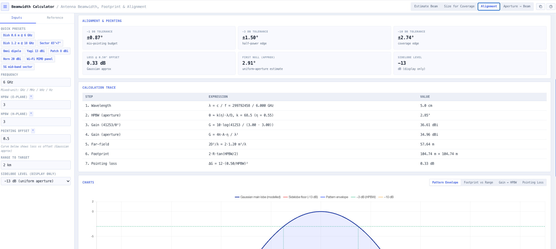
Top bar with the four task first modes (Estimate, Size for Coverage, Alignment, Aperture to Beam).

Walkthrough

See it working

Top bar with the four task first modes (Estimate, Size for Coverage, Alignment, Aperture to Beam).
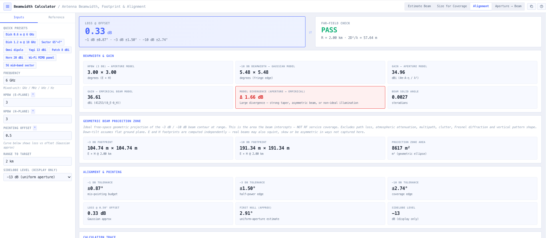
Footprint geometry at range with minus 3 dB and minus 10 dB contours and the tilted sector intersection.
Gaussian mis-pointing loss curve with markers at minus 1, minus 3, and minus 10 dB.

Top bar with the four task first modes (Estimate, Size for Coverage, Alignment, Aperture to Beam).

Overview

What the Beamwidth Calculator does

Antenna beamwidth sits between two extremes of antenna analysis. The textbook formulas (70 lambda over D for a uniformly illuminated dish, or 27000 over the product of E plane and H plane beamwidths for gain estimation) are simple but only approximate. Full wave electromagnetic simulation is precise but requires a model, software licence, and time none of which is available during early link sizing or installer mount specification work. Communication systems integrators need a middle ground. A practical calculator that uses the inputs they have on hand (gain, aperture, frequency, range) and returns the numbers they actually use (half power beamwidth, footprint at range, mount precision, far field distance) with honest caveats about approximation accuracy.

Read the full overview

The noIM₃ Beamwidth Calculator is that middle ground. Task first modes structure the workflow around what the engineer is doing rather than what equation they remember. Estimate Beam returns half power beamwidth (HPBW) from a gain or aperture input. Size for Coverage takes a target footprint diameter at a known range and returns the required HPBW, implied gain, and required aperture. Alignment converts beamwidth into pointing tolerance and a mis pointing loss curve, directly answering how precise does the mount need to be. Aperture to Beam handles the case where the physical antenna geometry is known and the question is what beam it produces.

Honest approximation handling is the differentiator. Gain is reported via both the aperture method (G equals 4 pi A eta divided by lambda squared) and the beamwidth method (G equals 27000 divided by the product of E plane and H plane HPBW in degrees), with a colour coded agreement badge. Differences of 10 to 20 per cent between the two are normal and the calculator surfaces the spread rather than hiding behind a single number. Far field validity is checked explicitly using the Fraunhofer distance 2 D squared over lambda. Pass or fail flag becomes actionable. When failing, the tool calls out that beamwidth and footprint values may be invalid in the near field and shows the minimum valid range. Mis pointing loss follows the standard Gaussian approximation delta G in dB equals 12 times (theta over HPBW) squared, plotted with markers at minus 1, minus 3, and minus 10 dB so mount specification, wind and sag budgeting, and installation tolerance assessment are all driven from the same plot.

Capabilities 9

Task first modes

Four modes structured around integrator workflows. Estimate Beam returns HPBW from gain or aperture. Size for Coverage takes a target footprint and range and returns required HPBW, gain, and aperture. Alignment converts beamwidth into pointing tolerance and mis pointing loss. Aperture to Beam takes physical antenna geometry and returns the resulting beam. The same physics is presented in the form that matches what the engineer is trying to do.

Dual gain cross check

Gain reported via both the aperture method G equals 4 pi A eta over lambda squared and the beamwidth method G equals 27000 over (theta E times theta H), with a colour coded agreement badge. Differences of 10 to 20 per cent are normal. The calculator surfaces the spread rather than hiding behind a single number, supporting honest design discussions and avoiding false precision in early sizing.

Far field validity check

Computes the Fraunhofer distance 2 D squared over lambda and compares it against the entered range. Pass or fail flag becomes actionable. When failing, the calculator calls out that beamwidth and footprint values may be invalid in the near field and shows the minimum valid range. Useful for antenna range measurements, near field exclusion checks, and confirming that link distances place the receive antenna in valid far field.

Mis pointing loss curve

Mis pointing loss computed as delta G in dB equals 12 times (theta over HPBW) squared (the standard Gaussian approximation), plotted with markers at minus 1, minus 3, and minus 10 dB pointing offsets. Useful for sizing mount precision, budgeting wind and sag, and assessing installation tolerance. Directly answers the integrator question how precise does my mount need to be.

Coverage sizing workflow

Given a target footprint diameter and range, the calculator returns the required HPBW, the implied gain, and the required circular aperture at the chosen efficiency. Closes the loop on whether the antenna is buildable in your size budget. Useful for sector antenna sizing, satellite ground footprint planning, and broadcast or distribution antenna design.

Aperture handling

Both circular (diameter D) and rectangular (width by height W and H) apertures supported. Output covers HPBW in E plane and H plane, footprint at range with axes labelled, and gain via both the aperture and beamwidth methods. Useful when the antenna is a dish, a horn, a patch array, or any directive structure with known physical aperture geometry.

Mixed unit text input

Input accepts mixed unit text such as 6 GHz, 1200 mm, 2 km, 18 inches, or 30 ft. The calculator parses unit suffixes automatically, matching the way integrators actually think and write rather than forcing field by field unit selection. Reduces input friction during fast lab and bench calculations.

Calculation trace and caveats

Every output is traceable. Wavelength derivation, HPBW formula chosen, gain by both methods, far field distance, footprint geometry, and pointing loss. Footprint output explicitly flags the geometric minus 3 or minus 10 dB contour as distinct from propagation coverage. Tilt projection is labelled flat ground. Useful for design documentation, customer reports, and engineering review where the assumptions need to be visible rather than hidden.

Browser only computation

Runs entirely in your browser. No antenna geometry, gain, or coverage data is submitted to a server. Useful for commercially confidential infrastructure planning, defence and security antenna design, and environments where information security policy prohibits sending engineering data to third party services.

Inputs and outputs

What goes in, what comes out

Inputs 9

  • Operating frequency in GHz, MHz, or wavelength in mm or cm or m
  • Antenna gain in dBi (Estimate Beam mode)
  • Antenna aperture diameter D for circular, or W and H for rectangular
  • Aperture efficiency eta as a percentage
  • Range to the target in metres or kilometres
  • Target footprint diameter (Size for Coverage mode)
  • Pointing offset angle theta in degrees (Alignment mode)
  • Mis pointing loss budget in dB (Alignment mode)
  • Antenna mount tilt angle for ground footprint projection

Outputs 13

  • Half power beamwidth (HPBW) in E plane and H plane
  • Minus 10 dB beamwidth
  • Footprint diameter at the configured range
  • Footprint area (with explicit caveat that this is the antenna pattern minus 3 or minus 10 dB contour, not propagation coverage)
  • Pointing tolerance to minus 1, minus 3, and minus 10 dB
  • Mis pointing loss curve versus angle
  • Gain via aperture method (4 pi A eta over lambda squared)
  • Gain via beamwidth method (27000 over theta E times theta H)
  • Agreement badge between the two gain methods
  • Fraunhofer far field distance 2 D squared over lambda
  • Far field pass or fail flag against the configured range
  • Required HPBW, gain, and aperture for a target coverage footprint (Size for Coverage mode)
  • Step by step calculation trace with formulas and intermediate values

Standards & methodology

  • IEEE 145. Standard definitions of terms for antennas
  • Balanis Antenna Theory analysis and design textbook formulations
  • Stutzman and Thiele Antenna Theory and Design textbook formulations
  • Standard 70 lambda over D approximation for circular aperture HPBW
  • Standard 27000 over (theta E times theta H) gain estimate from beamwidth (degrees)
  • Fraunhofer far field distance 2 D squared over lambda
  • Gaussian mis pointing loss approximation delta G in dB equals 12 times (theta over HPBW) squared

Use cases

When to use this tool

  1. 01Sizing a parabolic dish for a microwave or satellite backhaul link
  2. 02Specifying mount precision for a microwave installer
  3. 03Sizing a sector antenna for a target ground coverage area
  4. 04Validating that an antenna range measurement is in the far field
  5. 05Estimating mis pointing loss from wind and structural sag budgets
  6. 06Cross checking advertised antenna gain against published beamwidth
  7. 07Producing footprint diagrams for satellite ground coverage assessment
  8. 08Sizing horn antenna apertures for radar and instrumentation systems
  9. 09Specifying alignment tolerance during tower top antenna installation
  10. 10Producing teaching and training materials for antenna fundamentals
  11. 11Validating vendor antenna datasheet beamwidth claims against the underlying aperture
  12. 12Evaluating coverage trade offs between high gain narrow beam and lower gain wide beam alternatives

FAQ

Frequently asked questions

Not here? Ask us

How is HPBW estimated from gain or aperture?

For a uniformly illuminated circular aperture of diameter D, the standard approximation is HPBW in degrees equals 70 lambda over D. From gain, the standard approximation is gain in linear units equals 27000 divided by the product of E plane and H plane beamwidths in degrees, which inverts to HPBW estimation when one beamwidth is known or assumed equal to the other. The calculator uses these standard approximations and surfaces the formula chosen in the calculation trace so the assumptions are visible.

Why are there two gain methods and why do they disagree?

The aperture method G equals 4 pi A eta over lambda squared computes gain from the physical aperture and assumed efficiency. The beamwidth method G equals 27000 over (theta E times theta H) computes gain from observed beamwidths. Both are approximations. Real antennas have illumination tapers, sidelobes, and pattern asymmetries that the simple formulas do not capture, so the two methods typically disagree by 10 to 20 per cent. The calculator surfaces both with an agreement badge so the natural spread is visible rather than hidden behind a single false precision number.

What is the far field distance and why does it matter?

Beamwidth and footprint calculations assume the observation point is in the far field of the antenna, which means the radiation pattern has fully formed. The Fraunhofer far field distance 2 D squared over lambda is the standard threshold. Closer than this, near field effects dominate and the calculated beamwidth and footprint are not physically meaningful. The calculator computes this distance and flags whether the configured range is in valid far field.

How is mis pointing loss calculated?

Standard Gaussian approximation delta G in dB equals 12 times (theta over HPBW) squared, where theta is the pointing offset and HPBW is the half power beamwidth. This is exact at the half power point (theta equals HPBW divided by 2 gives delta G equals 3 dB). The calculator plots the curve out to large offsets and marks the minus 1, minus 3, and minus 10 dB points so the pointing tolerance budget is directly visible.

What inputs does the mixed unit text parser accept?

Frequency in Hz, kHz, MHz, GHz, or THz. Wavelength in mm, cm, m, or km. Aperture in mm, cm, m, in, or ft. Range in m or km. Examples include 6 GHz, 1200 mm, 2 km, 18 inches, 30 ft. The parser handles plural and abbreviated forms naturally so the input is accepted in whatever form is on the engineer datasheet or napkin sketch.

How is this different from the Parabolic Antenna Calculator?

The Parabolic Antenna Calculator focuses specifically on dish reflectors with deep parabolic reflector physics (gain, directivity, HPBW, effective aperture, Fraunhofer distance) and is the right tool when the question is what a particular dish does. The Beamwidth Calculator is the integrator workflow for any antenna shape (dish, horn, patch, sector, custom), structured around the integrator tasks (estimate, size for coverage, alignment, aperture to beam) rather than antenna type. Use the Parabolic Antenna Calculator for dish detail. Use the Beamwidth Calculator for general integrator tasks across any antenna.

How does this support installation and acceptance work?

Mount precision is sized directly from the mis pointing loss curve. Wind and structural sag budgets translate directly into dB cost via the same curve. Acceptance testing benefits from the explicit far field validity check so range measurements are not invalidated by near field artefacts. Footprint output supports satellite and sector coverage diagrams. Together they cover the antenna sizing, mount specification, and acceptance test workflows that integrators run repeatedly.

Does any data leave my browser?

No. The calculator runs entirely in your browser. No antenna geometry, gain, or coverage data is submitted to a server. Useful for commercially confidential infrastructure planning, defence and security antenna design, and environments where information security policy prohibits sending engineering data to third party services.

Free, no sign-up

Free to use, no sign-up needed.