Microwave Link Planning

Friis Transmission Calculator

Free space received power and link feasibility analysis from the Friis transmission equation. Compute received power from transmit power, antenna gains, frequency, and distance, with FSPL, EIRP, wavelength, and signal strength classification.

Overview

The Friis transmission equation is the most widely used result in RF engineering. It tells you how much of the power you transmit ends up at the receiver under ideal free space conditions, given the antenna gains at each end, the operating frequency, and the separation distance. Every link budget, every coverage estimate, every feasibility study starts with Friis. Get the inputs right and you have a defensible upper bound for the received power. Get them wrong and the rest of the design rests on a number that is silently a few orders of magnitude off.

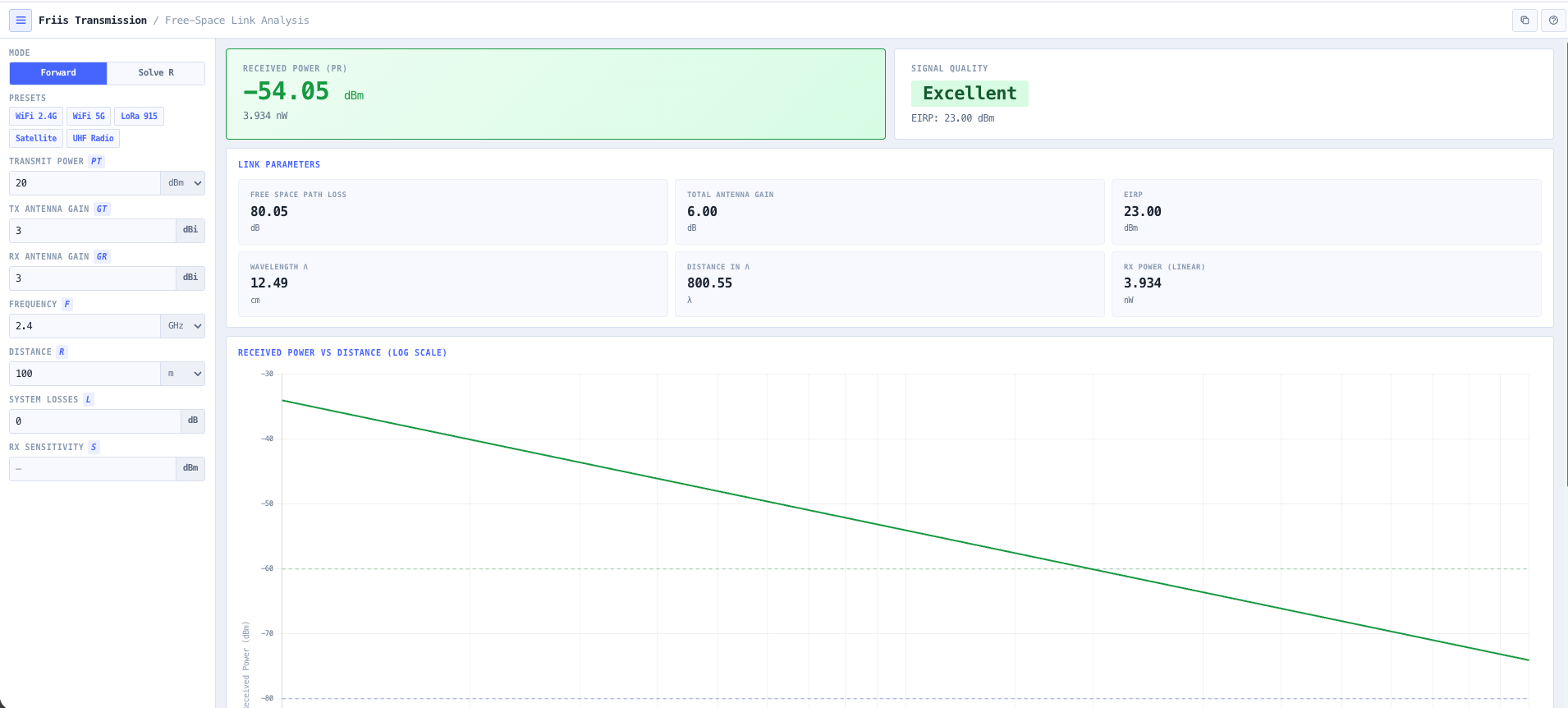
The noIM₃ Friis Transmission Calculator gives that upper bound in one workspace. The dB form of the Friis equation (Pr equals Pt plus Gt plus Gr minus FSPL minus system losses) is implemented directly. Inputs are transmit power in dBm, watts, or milliwatts, transmit and receive antenna gain in dBi, operating frequency in Hz, kHz, MHz, or GHz, separation distance in metres, kilometres, feet, or miles, optional system losses, and an optional receiver sensitivity. Output is received power in both dBm and watts, free space path loss in dB, effective isotropic radiated power, total antenna gain, wavelength at the operating frequency, and the separation distance expressed in wavelengths so the far field assumption is visible rather than implied.

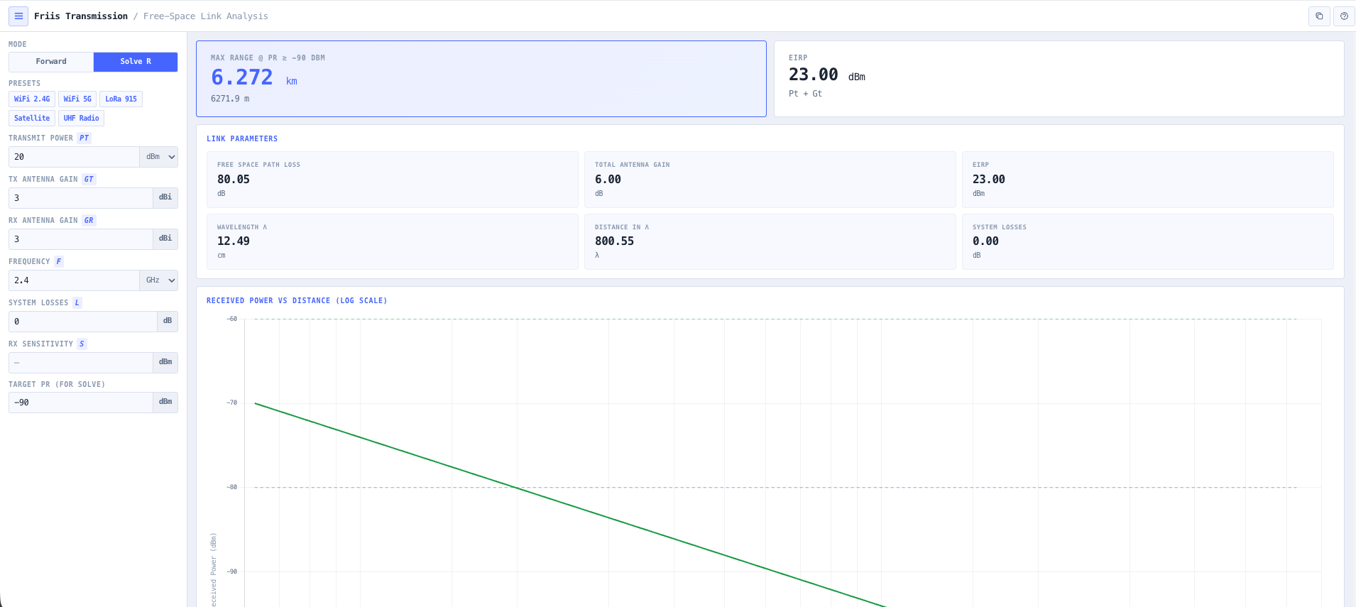
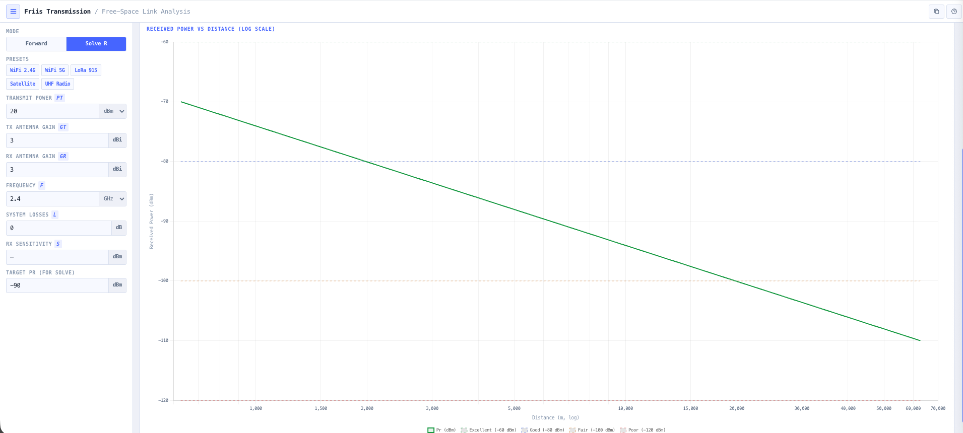
Two modes share the same inputs. Forward mode solves for received power; Solve-R mode inverts the equation and returns the maximum free space range at which the link stays above a target received power. Built in presets cover WiFi 2.4 GHz and 5 GHz access point links, LoRa 915 MHz IoT coverage, UHF radio paths, and a satellite link at geostationary slant range, so a usable answer is one click away. A five band signal quality classification (excellent, good, fair, poor, critical) gives an immediate qualitative feasibility read, a near field warning flags links too short for the Friis model to hold, and an interactive received power versus distance chart shows the inverse square fall off so the operating margin against the noise floor is intuitive.

Capabilities

Friis equation in dB form

Implements the classical Friis transmission formula in its dB form. Pr equals Pt plus Gt plus Gr minus FSPL. All link budget contributions are in decibels so the calculation is a straight read across rather than an exponential evaluation. Output covers received power in dBm and watts simultaneously.

Free space path loss

FSPL computed in the standard logarithmic form FSPL equals 20 log(d) plus 20 log(f) plus a frequency dependent constant. Output is in dB for direct subtraction in the link budget. Surfaces how propagation loss scales with both range and frequency, which is the right intuition for choosing between a 2.4 GHz and a 5 GHz link, or between a UHF and a microwave path.

EIRP and total system gain

Effective isotropic radiated power computed from transmit power plus transmit antenna gain, surfaced in dBm and watts. Total system antenna gain (Gt plus Gr) shown explicitly so the contribution of antennas at each end of the link is visible in the budget rather than buried inside the received power number.

Wavelength, electrical distance, and a near field warning

Automatic conversion of operating frequency to wavelength in metres, centimetres, or millimetres. Separation distance shown in wavelengths to surface electrical scale, and a near field warning is raised when the link is shorter than about ten wavelengths, where the Friis far field model loses validity. Useful for physically small antennas, near field exclusion checks, and any application where the wavelength to distance ratio matters more than the absolute distance.

Forward and Solve-R inverse modes

Forward mode solves for received power given the transmit power, antenna gains, frequency, distance, and system losses. Solve-R mode inverts the equation: given a target received power, it returns the maximum free space range at which the link stays at or above that target. Solve-R answers the coverage question directly rather than by trial and error on the distance field.

System losses and link margin

A system losses input in dB captures feeder cable, connector, and polarisation mismatch losses outside the free space path. Enter an optional receiver sensitivity and the calculator reports the link margin (received power minus sensitivity) directly, giving an immediate read on whether the link closes and by how much. A negative margin means the link will not close under free space conditions.

Signal quality classification

Qualitative classification of the received power against typical receiver sensitivity thresholds. Returns one of five bands (excellent, good, fair, poor, critical) so non specialist stakeholders can read the result without converting dBm to a feeling. Useful for WiFi, LoRa, UHF radio, and satellite style feasibility checks.

Received power versus distance chart

An interactive chart plots received power against separation distance on a logarithmic axis under the inverse square law behaviour of free space propagation, with the signal quality thresholds and the optional receiver sensitivity drawn as reference lines. Useful for understanding the rate at which margin is consumed by range and for producing intuitive visuals for design reviews and customer reports.

Wireless system presets

Quick select presets for WiFi 2.4 GHz and 5 GHz access point links, LoRa 915 MHz IoT coverage, a UHF radio path at 450 MHz, and a satellite link at geostationary slant range. Manual entry remains available for unusual configurations including amateur radio, IoT, telemetry, microwave point to point, and short range links.

Browser only computation

Runs entirely in your browser. No transmitter power levels, antenna data, or link parameters are submitted to a server. Useful for commercially confidential infrastructure work or environments where information security policy prohibits sending engineering data to third party services.

Standards & methodology

  • Friis transmission equation (Friis 1946)
  • IEEE 145. Standard definitions of terms for antennas
  • ITU R P.525. Calculation of free space attenuation
  • ITU R P.341. The concept of transmission loss for radio links

When to use this tool

  • WiFi 2.4 GHz and 5 GHz link feasibility and rough range estimation
  • LoRa and IoT coverage estimation at 915 MHz
  • UHF and VHF radio system received power evaluation
  • Satellite link margin estimation under free space approximation
  • Microwave point to point feasibility analysis before detailed link budget work
  • Educational demonstrations of the inverse square law and free space propagation
  • Sanity checking a vendor proposed link budget against the underlying physics
  • Producing back of envelope feasibility numbers during early site planning
  • Comparing two candidate frequency bands for the same path
  • Evaluating maximum operating distance for a specified receive sensitivity
  • Producing teaching examples and reference calculations for RF engineering courses
  • Quick what if analysis on the impact of antenna gain or transmit power changes

Is this the right tool for you?

Reach for the Friis Transmission Calculator in any of the following situations.

  • You are evaluating a WiFi 2.4 GHz or 5 GHz link between two buildings and want a fast feasibility check before commissioning a survey or running detailed link planning.
  • You are sizing a LoRa or IoT deployment at 915 MHz and need received power versus range so you can plan gateway placement against the device receiver sensitivity.
  • You are designing a UHF or VHF radio path and want a free space upper bound on the received power before adding terrain, vegetation, and clutter losses to the budget.
  • You are estimating satellite link margin under a free space approximation and need EIRP, FSPL, and received power for the uplink or downlink as a sanity check.
  • You are doing early stage microwave point to point feasibility analysis and want the free space numbers before committing to a full ITU P.530 link planning exercise.
  • You are training new RF engineers in fundamentals and want a teaching tool that shows how received power scales with range, frequency, and antenna gain visually.
  • You are sanity checking a vendor proposed link budget and want an independent Friis calculation against the underlying free space physics.
  • You are comparing two candidate frequency bands for the same path (for example 2.4 GHz versus 5 GHz, or 900 MHz versus 5.8 GHz) and want a like for like received power comparison.
  • You are evaluating the maximum operating distance for a specified receive sensitivity and want the range at which received power equals the threshold.
  • You are producing back of envelope feasibility numbers during a site planning meeting and need fast, defensible received power estimates.
  • You are validating that a candidate link will close under free space conditions before investigating whether terrain, multipath, or rain will close the margin.
  • You are a contractor or consulting engineer producing a customer feasibility report and need free space upper bound numbers that the customer can verify.
  • You are evaluating the impact of changing transmit power, antenna gain, or frequency on link feasibility before committing to the change.
  • You are an amateur radio operator estimating coverage from a portable or mobile setup and want a fast received power estimate at the other end of the path.
  • You are operating under a security regime that prohibits sending design data to third party services and need a Friis calculator that runs entirely in your browser.

Frequently asked questions

What is the Friis transmission equation?

The Friis transmission equation (Friis 1946) gives the received power at a receive antenna when a transmit antenna radiates a known power across a free space path. In its dB form it is Pr equals Pt plus Gt plus Gr minus FSPL, where Pr is received power, Pt is transmit power, Gt and Gr are the transmit and receive antenna gains in dBi, and FSPL is the free space path loss in dB. It is the foundational result used in every link budget.

When does free space actually apply?

Friis assumes ideal line of sight conditions with no obstructions, no terrain, no atmospheric absorption, no multipath, and that both ends of the link are in the far field of each other antenna. It is the right model for satellite links above the atmosphere, for short range line of sight links, and as the upper bound starting point for any link budget. For terrestrial links over significant range, you usually need to add additional propagation effects (rain, gas absorption, diffraction over terrain, multipath, clutter) that the noIM₃ Link Planner handles to ITU P.530.

How is FSPL calculated?

Free space path loss in dB equals 20 log(d) plus 20 log(f) plus a frequency dependent constant. For d in metres and f in MHz, FSPL equals 20 log(d) plus 20 log(f) minus 27.55. For d in kilometres and f in GHz, FSPL equals 20 log(d) plus 20 log(f) plus 92.45. The calculator uses the appropriate form for your input units and reports FSPL in dB ready for direct subtraction in the link budget.

What does the signal quality classification mean?

A qualitative classification of the received power against typical receiver sensitivity thresholds. The calculator returns one of five bands so non specialist stakeholders can read the result without learning to interpret dBm: excellent at or above minus 60 dBm, good from minus 60 to minus 80 dBm, fair from minus 80 to minus 100 dBm, poor from minus 100 to minus 120 dBm, and critical below minus 120 dBm. The thresholds are a generic benchmark for common applications. For a precise feasibility decision, enter the actual receiver sensitivity and read the dB link margin directly.

What is Solve-R mode?

Solve-R inverts the Friis equation. Instead of computing received power at a fixed distance, you enter a target received power (typically a receiver sensitivity threshold) and the calculator returns the maximum free space range at which the link stays at or above that target, honouring the configured transmit power, antenna gains, frequency, and system losses. It answers the coverage planning question directly rather than by trial and error on the distance field.

How is this different from the Free Space Path Loss Calculator?

The FSPL Calculator focuses solely on the propagation loss in dB as a function of distance and frequency. The Friis Transmission Calculator extends that to the full free space link, returning received power, EIRP, total antenna gain, and signal strength against a known transmit power and antenna pair. Use FSPL when you only need the loss number. Use Friis when you need the received power and link feasibility.

How is this different from the Link Budget Calculator?

Friis is the free space upper bound. The Link Budget Calculator extends the analysis to a full operational link budget including feeder loss, miscellaneous losses, fade margin, atmospheric and rain attenuation, and link availability. Use Friis for fast feasibility and teaching. Use the Link Budget Calculator for the full operational budget that goes into a design package.

Does any data leave my browser?

No. The calculator runs entirely in your browser. No transmit power, antenna gain, frequency, or distance values are submitted to a server. Useful for commercially confidential infrastructure work or environments where information security policy prohibits sending engineering data to third party services.

Can I use it for satellite links?

Yes, as a free space approximation. Satellite links above the atmosphere are very close to free space, so Friis gives a good first approximation of the link margin. For precision satellite link work you would also need to account for atmospheric loss (P.676 gas absorption), rain attenuation (P.618), and antenna pointing loss, none of which are inside Friis. Use Friis for the upper bound and feasibility, then layer additional losses on top.