What are the three spacing ceilings and which one usually binds?
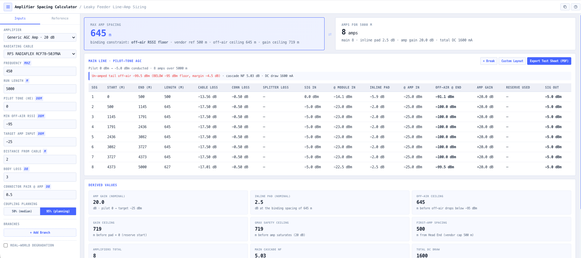
The calculator runs three independent constraints: (1) off-air RSSI ceiling — segment length where conducted minus coupling minus distance falloff minus body loss minus connector pair just meets the user-set RSSI floor; (2) amp-gain target ceiling — segment length where the inline pad runs to zero and the gain block starts consuming reserve; (3) Gmax safety ceiling — segment length where the amp saturates. The tightest binds, named in the hero card. In realistic mining (95 % planning coupling, 5 m listener distance, 3 dB body loss) the off-air ceiling almost always binds. Vendor handbook spacing numbers are the amp-gain ceiling, not the off-air ceiling, and are recovered only when you strip body loss, set listener distance to the 2 m reference, and use the 50 % median coupling.
How many amps will the tool say I need?
Every segment in the chain ends with an amplifier — the model has no un-amped tail. So if the main line has 15 segments and a branch has 4 segments, the procurement number on the Amps for Run hero card is 19 amps total. The split between main and branches is shown alongside the total so you can read both numbers at a glance. This matches the real install: every amp boundary is a piece of hardware in the BOM.
Why generic AGC amplifier classes instead of vendor presets?
The tool is intentionally vendor-agnostic. The three AGC classes (20 / 25 / 30 dB max gain with 3 / 4 / 5 dB reserve, 200 / 250 / 300 mA DC, 5 dB NF, 33 dBm OIP3) cover the realistic spread of mining and tunnel line amps without locking the user to a single product line. Vendor-specific datasheet variations sit downstream in the full Leaky Feeder Designer canvas environment. This calculator focuses on the physics that drive the quote — cable loss, coupling, off-air budget, inline pad — which are nearly identical across vendor implementations of the same AGC gain class.
What is the inline pad and why is it surfaced separately?
Every amplifier module is [input pad] → [AGC gain block] → [output]. The pad attenuates the cable-side signal so the gain block sees the user-set target input level (typical −25 to −30 dBm for mining). The gain block then applies (pilot − target) of gain to restore the chain to pilot at the output. The pad value per segment is the number the field tech actually dials in at install — so it gets its own column in the trace and in the PDF test sheet, with the Cable Loss and Conn Loss columns alongside so the dial-in math is visible.
Why does coupling-loss matter so much, and why default to 95 %?
Manufacturer datasheets publish coupling loss at two planning levels: 50 % (median — half the points along a long cable have ≤ this loss) and 95 % (planning — 95 % of points have ≤ this loss). The 95 % value is typically 6–10 dB worse than the 50 % value (8 dB on RFS RADIAFLEX and CommScope RADIAX at 450 MHz). The 95 % value is what you size for in real mining design because the field experience is the worst-case slot pattern, not the median one. The Coupling Planning toggle exposes both — set it to 50 % to recover the lab numbers, leave it on 95 % for the honest field design.
How does coupling change with frequency?
Coupling loss drops roughly 2.5 dB per decade with rising frequency — smaller wavelength means the slot pattern radiates more efficiently. The calculator applies this correction to the stored 450 MHz reference value: CL(f) = CL(450) − 2.5 · log₁₀(f / 450). Verified against the RFS RCF78 2024 datasheet across 75 MHz to 2700 MHz to ±0.5 dB. Below 450 MHz the correction increases coupling (conservatively tightening VHF mining spacing); above 450 MHz it decreases coupling slightly.
How do the custom segment layouts work?
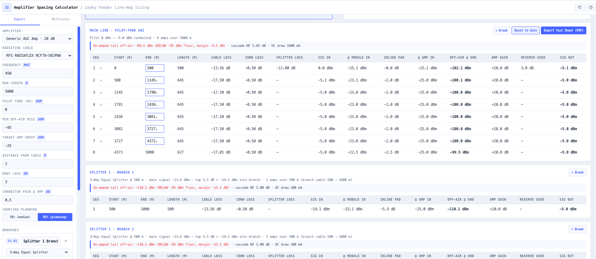
Click Custom Layout on the Main Line section to make each segment's End cell editable. Start of the next segment chains automatically and every dependent value (cable loss, connector loss, inline pad, off-air RSSI, amp gain, reserve) recomputes live. Use + Break on any chain header (main or a branch) to insert another amp position; click the × on any row to remove one. Custom layout state is per-chain — main and each branch carry their own boundaries so amp positions can be pinned against real drift access points and equipment niches.
How are branch segment positions displayed?
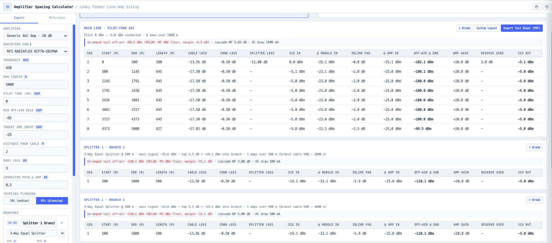
In Head-End-relative (mine-run) coordinates. A branch tapped at 500 m on the main run with a first segment of 350 m reads 500 → 850 m in the Start / End columns (not 0 → 350). The field tech walks a single cable-length-from-HE axis across the whole network. The branch chain title carries the explicit cable-axis span (e.g. "branch cable 500 → 1000 m") so the coordinate system is self-documenting in both the UI and the PDF test sheet.
What does the PDF test sheet contain?
A landscape A4 commissioning record matching the noIM₃ HF Link Report design system — no cover page, just one or more landscape pages of segment-table data ready to print. The header strip carries project / site / technician / date and the full design parameter set (amplifier class, cable, frequency, pilot, target amp input + gain, RSSI floor + distance, body / connector / coupling). Below the strip every chain renders its segment table with 12 columns: Seg # · Start (m) · End (m) · Length (m) · Cable Loss (dB) · Inline Pad SET (dB) · Expected @ Amp In (dBm) · Expected Off-Air @ End (dBm) · Measured @ Amp In (dBm) · Measured Off-Air @ End (dBm) · Pass / Fail · Notes. The four measured columns are amber-tinted so the printed sheet visually signals what the tech needs to write. Auto-paginates with the table header repeated on subsequent pages.
Does the calculator do intermodulation, DC voltage drop, or 3D coverage prediction?
No. This calculator is intentionally scoped to spacing, conducted signal level, inline pad sizing, off-air RSSI, cascade noise figure, and total DC current draw. Full intermodulation analysis (IM3 with downlink and uplink passband filtering at every amplifier and head end), bidirectional uplink and downlink, multi-carrier composite power tracking through the cascade, DC power feed solver, and over-the-air mobile-radio coupling sit in the dedicated Leaky Feeder Designer canvas environment. 3D coverage prediction with terrain and structure loss sits in the Leaky Feeder 3D Coverage tool. The Amplifier Spacing Calculator is the back-of-envelope feeder into those workflows and the commissioning record they sign off against.
How is cascade noise figure computed?
Per chain using the Friis formula with each amplifier's actual AGC gain block setting (= pilot − target input + reserve consumed on that segment), not the vendor Gmax. Feeding Gmax to Friis under-states cascade NF because lower per-stage gain raises the noise contribution of downstream stages. The reported number reflects the segment pattern shown in the trace, not a best-case floor.
Where do the cable K₁ / K₂ and coupling values come from?
Every cable in the library is sourced from a 2023–2024 manufacturer datasheet. K₁ / K₂ longitudinal loss coefficients are least-squares fitted across the published frequency points to ±0.1 dB / 100 m. Coupling losses are stored at the 50 % / 95 % planning levels at the cable's reference frequency, with provenance metadata (datasheet source, revision date, IEC test standard, last review date) stored alongside in the JSON cable database. The library covers RFS RADIAFLEX (RCF12, RCF78, RCF78-MSHA, RLF114, RLKW114), CommScope RADIAX (RXL-12, RXL-78, RXL-114), and Times Microwave LMR (LMR-600, LMR-900 — non-radiating feeders).
Does any of my network plan data leave the browser?
No. The calculator runs entirely in your browser. No amplifier class choice, cable selection, run length, branch topology, segment layout, commissioning measurement, or any other data is submitted to a server. This matters when the network plan is operationally sensitive, commercially confidential, or covered by an information security policy that prohibits sending raw infrastructure data to third party services.